Simulating the early Universe on a table top Quantum Simulator

By: Shaurya Bhave

Authors: Bo Song¹, Shovan Dutta¹, Shaurya Bhave¹, Jr-Chiun Yu¹, Edward Carter¹, Nigel Cooper² & Ulrich Schneider¹

Institution: 1) Cavendish Laboratory, University of Cambridge, Cambridge, UK
2) Department of Physics and Astronomy, University of Florence, Sesto Fiorentino, Italy.

Manuscript: Published in Nature Physics [4]

The natural world is host to several systems that exist in one or more phases. These phases are typically separated by a transition, often triggered by thermal fluctuations. A few prominent examples are phases of water, ferromagnetism in solids, and superconducting phases in strongly interacting systems such as high-temperature superconductors. These phases are typically separated by a transition and can typically be classified as either discontinuous or continuous.

Whether the transition is discontinuous or continuous depends on the path taken to change over from one state of the system to another. This is illustrated in Fig. 1, where the initial state changes seamlessly to the other in the case of a continuous one.

This is usually reflected in continuous change of the order parameter as parameters are swept through the transition point.

A discontinuous transition is characterized by a sudden change in the order parameter as the transition is crossed. The lack of a smooth change results in a phenomenon known as metastability (see Fig. 1). Metastability is the tendency of a global phase to persist despite crossing the transition point, indicating the existence of two stable equilibrium points.

Typically, these phase transitions are classical, as they are caused by thermal fluctuations. The most familiar example is the phase transitions of water. There also exist more complex transitions, such as the ferromagnetic to paramagnetic transition and the transition responsible for superconductivity.

The microscopic behaviour of the latter two systems is determined by quantum mechanics. However, the transition itself is classical. It is the result of thermal fluctuations within the system, as the temperature is reduced below a critical point.

A further distinction can be made between phase transitions that are driven by thermal fluctuations and those driven by quantum fluctuations. The latter are referred to as quantum phase transitions. Quantum phase transitions occur close to T = 0, and are mostly seen in degenerate quantum degenerate matter, such as the electron gas in metals.

Many studies usually focus on continuous phase transitions, as they are the most common form of quantum phase transitions. However, discontinuous transitions have been gaining interest for their relevance in the evolution of the early universe, where some studies suggest that the universe evolved from a hot plasma to its current state by multiple phase transitions [1, 2]. Various models have been proposed, which contend that these transitions were discontinuous; they occurred through the decay of a metastable state [3].

The study, carried out by lead author Bo Song [4], realized a quantum system which hosts a metastable state and displays a discontinuous phase transition. In this experiment, they tune this quantum phase transition from a continuous transition to a discontinuous transition and demonstrate the metastability of this state. This work builds on previous proposals for using ultracold atoms as a table top simulator of the early universe [5, 6] and opens the possibility to study the quantum decay of metastable states.

A table top Quantum Simulator

The aim of a quantum simulator is to study the behavior of a system governed by the laws of quantum mechanics such as solid-state systems. Often, the phenomenon of interest in these systems is clouded by unwanted effects, such as those of temperature and impurities in the case of metals. Due to these challenges in traditional solid-state experiments, one can instead use a simulation (to capture the same principal results).

However, simulating these on classical computers becomes difficult, because the Hilbert space needed to encode these computations increases exponentially with the size of the system.

This motivates the need for a quantum simulator. These can be of two types: digital or analog. Digital simulators decompose the evolution of the system into a series of operations called quantum gates (akin to logic gates). These gates are then implemented on a quantum computer – an assembly of qubits.

An alternative approach is to create a different physical system which is governed by quantum mechanics. This is where one creates an analogous system whose Hamiltonian maps onto the system you want to study. One example of an analog simulator ultracold atoms in optical lattices, which naturally realize the physical characteristic of electrons in periodic solids. It should be noted that digital simulator platforms- such as superconducting circuits [7] – have also been used in similar manners to implement lattice type physics.

An analog simulator is engineered to be highly controllable, and free of any unwanted effects. The high tunability gives the experimenter full control over the critical parameters of the Hamiltonian. This allows the experimenter to directly observe quantum states and ground state phases. In traditional solid-state experiments, signatures of different phases are probed indirectly, but with quantum simulators, one can directly observe phase transitions like magnetism [8] and Mott insulating phases [9].

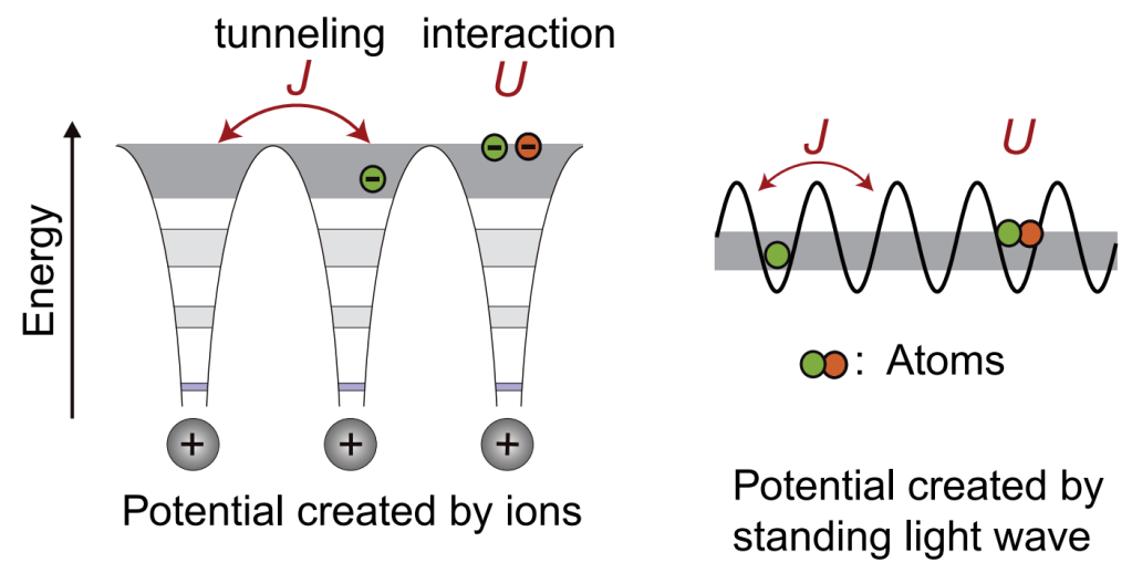
This experiment uses a Bose degenerate gas of 87Rb atoms – a Bose Einstein condensate (BEC) – that is loaded in an optical lattice. This degenerate gas of atoms mimics the role of the Fermi degenerate electron gas in metals, and the wells of the lattice are analogous to the potential wells of ions in metals (see Fig. 2). The larger mass and size of atoms, as compared to electrons, means the relevant quantum dynamics occur more slowly and can thus be directly observed. The only caveat is that the temperature of the gas needs to be close to absolute zero (around a few 10 nK).

A BEC loaded in a 1D optical lattice (see Fig. 3) can be in one of two ground state phases: an extended and conducting superfluid phase, or a localized Mott insulating (MI) phase.

A quantum phase transition occurs between these phases as the ratio of tunnelling to onsite interaction is changed. This is usually done by either adjusting the height of the lattice potential, or by adjusting the scattering length of the atoms by means of Feshbach resonance. When interactions dominate, the atoms are pinned to each site and tunnelling is suppressed. As the interactions are reduced, the tunnelling becomes dominant, and the atomic system is now extended. This is an example of a continuous phase transition which occurs in the ground band of the lattice.

Song demonstrates that this phase transition can be made discontinuous by employing a periodic drive to the 1D lattice system. Resonantly shaking the 1D lattice system couples the ground and the first excited band. The larger tunnelling in the first excited band causes an initially prepared Mott insulator to melt into a superfluid state. The negative curvature of the first band causes the condensate to occur at the edges of the Brillouin zone (k = ± π), earning the state the name: π – superfluid (π – SF, see Fig. 4).

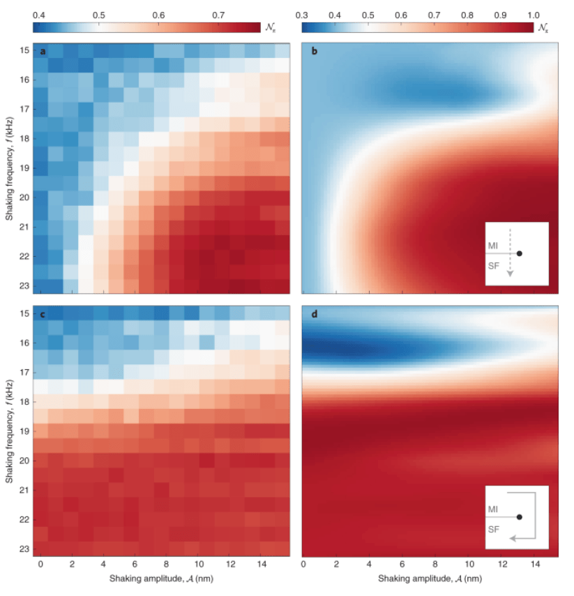
The teams map out the phase diagram of this driven system as a function of the driving parameters: driving strength and the frequency (see Fig. 5). The driven system is described by an effective Hamiltonian. The primary parameters of this Hamiltonian are, detuning from interband resonance, which is controlled by the drive frequency, and the coupling to the drive, which is controlled by the drive strength. The ground state is determined by the competition between these two parameters, in a manner analogous to tunnelling and interaction strength in the static system.

The phase diagram displays the two phases (MI or π-SF) that are separated by a discontinuous and continuous transition depending on the driving strength. The team identifies the discontinuous region by demonstrating the metastability associated with the discontinuous transition.

This experiment represents the first directly observable quantum first order phase transition. By realizing a system with a transition whose character can be tuned to be discontinuous, this study lays the foundations for the creation of metastable states. The unique experimental set up will enable the observation of the quantum decay process of these metastable states.

References:

[1] “Quantum Phase Transitions”, S. Sachdev, Phys. World, 12, 4 (33)
[2] “Some implications of a cosmological phase transition”, T. W. Kibble, Phys. Rep. 67, 183 – 199 (1980)
[3] “Fate of the false vacuum: semiclassical theory.”, S. Coleman, Phys. Rev. D. 15, 2929 (1977)
[4] “Realizing discontinuous quantum phase transitions in a strongly correlated driven optical lattice”, Bo Song et al, Nature Physics, 18, 259–264 (2022)
[5] “Fate of the false vacuum: towards realization with ultra-cold atoms.” ,O. Fialko et al, EPL 110, 56001 (2015)
[6] “The universe on a table top: engineering quantum decay of a relativistic scalar field from a metastable vacuum.”, O. Fialko et al, J. Phys. B: At. Mol. Opt. Phys. 50, 024003 (2017)
[7] “Disorder-assisted assembly of strongly correlated fluids of light”, B. Saxberg et al, Nature 612, 435–441 (2022)
[8] “A cold-atom Fermi-Hubbard anti-ferromagnet”, A. Mazurenko et al, Nature, 545, 462 – 466 (2017)
[9] “Quantum phase transition from a superfluid to a Mott insulator in a gas of ultracold atoms”, M. Greiner et al, Nature, 415, 39-44 (2002)
[10] “Interacting Fermionic Atoms in Optical Lattices – A Quantum Simulator for Condensed Matter Physics”, U. Schneider
[11] “Quantum Simulators”, I. Buluta and F. Nori, Science, 326, 5949, 108-111 (2009)