Title: High-fidelity two-qubit gates on fluxoniums using a tunable coupler
Authors: Ilya N. Moskalenko, Ilya A. Simakov, Nikolay N. Abramov, Alexander A. Grigorev, Dmitry O. Moskalev, Anastasiya A. Pishchimova, Nikita S. Smirnov, Evgeniy V. Zikiy, Ilya A. Rodionov & Ilya S. Besedin
Institutions:
- National University of Science and Technology ‘MISIS’, Moscow, Russia; Russian Quantum Center, 143025, Skolkovo, Moscow, Russia
- Moscow Institute of Physics and Technology, 141701, Dolgoprudny, Russia
- Dukhov Research Institute of Automatics (VNIIA), Moscow, 127055, Russia
- FMN Laboratory, Bauman Moscow State Technical University, Moscow, 105005, Russia
Manuscript: Published 08 November 2022 on Nature
Note: This is part of a series of articles written as final projects for Physics 438b at USC.
Background and Motivation
Currently, in the realm of quantum computers and quantum devices, there is an ongoing search for better system architectures to improve reliability and mitigate information loss when performing operations on qubits. These efforts are essential for the advancement of quantum computing, as qubits are inherently fragile and susceptible to decoherence and other unwanted effects. Decoherence occurs when a qubit interacts with its environment in such a way that the original state becomes mixed or entangled with the states of its surroundings. If decoherence occurs, we lose valuable information about a system and cannot perform high-precision operations.
Many recent quantum processor designs involve the implementation of two-qubit gate systems, where transmon qubits serve as the fundamental element upon which quantum gates operate. In quantum circuits, these gates serve as the building blocks that perform operations on the qubits. Transmon qubits, created by a small superconducting island (an island being a region of some superconducting material) connected to a reservoir by a Josephson junction, have been extensively researched in the past decade and are a popular choice for quantum computing. They exhibit low levels of decoherence in comparison to other qubit architectures, enabling transmons to maintain a certain quantum state for a longer period, thus allowing for more reliable operation results. Even so, transmon qubits still have some information loss; for example, they can have lower gate fidelities, which are a measure of how accurately the qubit performs as a quantum gate. Although some transmon qubit systems have almost perfect fidelity (two-qubit systems have been shown to have gate fidelities of ~99.5% according to various demonstrations), there are still other concerns. Crosstalk, the phenomenon in which a quantum state of one qubit affects another, leads to computational errors and decreases the reliability of transmon qubits. Transmon qubits are particularly susceptible to a specific type of crosstalk known as static ZZ interaction, which is a specific type of persistent and undesired coupling that can lead to decoherence and qubit frequency/state shifts.
Because of these challenges, alternative two-qubit architectures with fewer situations for decoherence to occur along with higher gate fidelities are being explored. One type of qubit, known as a fluxonium, is gaining traction in quantum processors and is the subject of this article. Specifically, a fluxonium two-qubit gate system where the qubits are paired to a tunable capacitive coupler could be a novel way of developing scalable NISQ (Noisy Intermediate-Scale Quantum) devices.
Fluxonium Qubits
Fluxonium qubits consist of a superconducting loop—different from transmon’s superconducting island—interrupted by a Josephson junction. The Josephson junction has a weak insulating barrier that allows pairs of electrons (called Cooper pairs) to tunnel through it, and through this tunneling, the qubit’s quantum state can be manipulated. When a current is applied to the superconducting loop, it creates a magnetic flux that becomes trapped by the junction. This magnetic flux is quantized, meaning it is discrete in value and can exist only in certain allowed states. These discrete states form the basis of the quantum states of the qubit, and they can be manipulated using quantum gates to perform operations in a quantum computer.
Just like transmon qubits, fluxonium qubits have high gate fidelities and long coherence times, allowing them to maintain a state for a long time without decaying to another state. Fluxonium qubits also have a better level of control over states versus the transmon qubits. Importantly, these qubits are characterized by a lower frequency than transmon qubits. These (resonant) frequencies dictate how the qubit can be manipulated when specific control signals are applied. Fluxonium qubits are also more resistant to information loss and noise, although static ZZ interactions are still a critical issue.
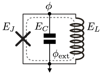
 ), the central conductor (
 ), and the inductor (
 ). The addition of the inductor is basically a step up from the transmon qubit.4
Adding a tunable coupler…
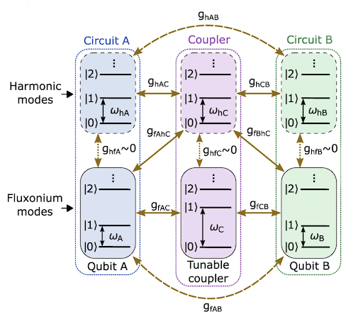
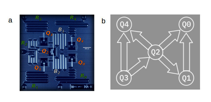
In order to simultaneously increase the gate fidelity and suppress static ZZ interaction in the two-qubit gate processor, the researchers created a processor (see Figure 3) featuring two modified fluxonium circuits (with extra harmonic modes so, therefore, more resonant frequencies) with a central tunable capacitive coupler in which the coupler’s frequencies are controlled by individual fast flux bias lines that are directly electrically connected (galvanically). These are just a type of superconducting circuit that controls the magnetic flux in a qubit. The flux control/bias lines are prone to issues if not developed and implemented carefully; the most relevant issues being attenuation and filtering. Attenuation refers to the loss of signal strength as a control signal transfers through a flux control line which affects the accuracy of the control (since it is difficult to get the sought-after control signal to the qubit). Filtering refers to the removal of unwanted frequencies and noise: if not well designed, it can also remove frequencies from the control signal, which affects reliability. In the case of this article, the individual galvanization allows for independent control of magnetic flux in each bias line. This method of implementing tunable coupling in a quantum computer using capacitive coupling relies on the phenomenon of charge transfer between two objects due to their proximity, to control the interactions between qubits. In this architecture, the qubits are arranged in a specific configuration that allows for this capacitive coupling. By making small adjustments to the distance between the qubits (as well as the size and shape of what they are made of), it is possible to control the strength of the capacitive coupling between them. Just as the qubits have their own frequencies (Qubit A: 


Now, with some careful manipulation to reduce the degrees of freedom of the system, the effective-low energy Hamiltonian of this two-qubit processor becomes:

Notice that this Hamiltonian includes two ‘qubit terms’ and some additional ones as well; the third term relates to the coupling, and the fourth term relates to the ZZ interaction!
Time for Quantum Gates
From here, universal gates, which are a set of logical operations that can be used to create any other logical operation, were implemented on the processor using specific pulse sequences. Specifically, the CZ gate and a variation of the iSWAP gate (called the √iSWAP-like gate) were chosen for this purpose; both of these choices derive from what is known as the fSim family. The fSim family is a group of quantum algorithms based on the original fSim (fermionic simulation) algorithm which simulates several different quantum systems, including gates. fSim can be represented with a matrix in the 

Where the swap angle 

With this in mind, the qubit-qubit coupling term 


 vs /2pi. Notice that there is a region of steadiness from -0.4 to 0.4 flux offset .2
The researcher’s √iSWAP-like gate (with 


The CZ (controlled-Z) gate, which was also included in testing because of various precision-related drawbacks the √iSWAP-like gate alone has, was created with two fSim (
Next, using the coupler flux bias lines, researchers introduced flux pulses that enabled them to precisely modulate the flux. This flux modulation allowed for the qubits to come into resonance. As mentioned previously, these fluxonium qubits operated at a lower frequency than transmon qubits, which allowed the researchers to perform more operations within a period of time without the qubit decaying to a lower state.
Experimental Results
After the implementation of both of these processes, through experiment, it was discovered the static ZZ interaction was almost entirely eliminated (less than 1 kHz remaining!) over a wide range of magnetic fluxes because of the addition of the tunable coupler and the ability to precisely control
As for gate fidelities of the CZ and √iSWAP-like gates, each was verified using a method called cross-entropy benchmarking (XEB).3 XEB is an algorithm that involves preparing a particular quantum state, performing a specific set of manipulations via various measurement operators, and then analyzing the output of said manipulations probabilistically in comparison to the same state and operations on another (reference) processor/system. In relation to XEB, a parameter called “circuit depth,” which is easiest related to the complexity of a circuit: the greater the depth, the more difficult and resource-consuming the system may be to implement on a quantum computer. Typically it is best practice to minimize this value, although experimentally it was varied to show how the fidelity exponentially decreased as circuit depth increased.
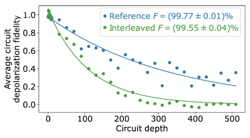
For the √iSWAP-like gate, its resulting gate fidelity was measured to be F = (99.55 ± 0.04)%, as Figure 5 represents with interleaved F. Meanwhile, the CZ gate fidelities were tested using different numbers of CZ gates in a linear sequence; experimentally, the greater the number (n) of CZ gates in sequence, the lower the average circuit depolarization fidelity (see Figure 6). For a single CZ gate alone, the fidelity was measured to be F = (99.22 ± 0.03)%.
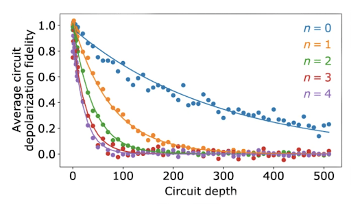
 corresponds to the number of CZ gates in a linear sequence.2
Conclusion
In confirming significant static ZZ suppression as well as gate fidelities greater than previously recorded in comparison to processors composed of transmon qubits, it is evident that this processor architecture composed of fluxonium qubits with a tunable capacitive coupler shows that fluxonium qubits are a promising alternative to the popular transmon option in regards to the creation of a quantum processor in which qubits remain in a single state for a longer period of time while maintaining resistance to crosstalk. These two characteristics are essential for the development of future scalable quantum computers. Hopefully, given this success, fluxonium qubits will receive greater attention and experimentation in the near future.
References
1 Moskalenko, I. N., Besedin, I. S., Simakov, I. A. & Ustinov, A. V. Tunable coupling scheme for implementing two-qubit gates on fluxonium qubits. Appl. Phys. Lett. 119, 194001 (2021).
2 Moskalenko, I.N., Simakov, I.A., Abramov, N.N. et al. High fidelity two-qubit gates on fluxoniums using a tunable coupler. npj Quantum Inf 8, 130 (2022).
3 Arute, F. et al. Quantum supremacy using a programmable superconducting processor. Nature 574, 505–510 (2019).
4 Nguyen, L. B. et al. The high-coherence fluxonium qubit. American Physical Society 9, 4 (2019).


 ; here we take the value of
  . Their Bell states are thus written as:

 and
and  correspond to
  is the Fermion state (also shown as the 4th state in (a) of


 refers to all of the possible OAM states. Note that the OAM state here doesn’t have to be a Bell state, but only one of the Bell states will give an exchange phase of π. For a Boson state in OAM, exchanging the two photons does not make a difference on the overall state, thus ΦO should be 0; on the contrary, for a Fermion state the exchanged state acquires a minus sign, so ΦO should equal to π (exchange anti-symmetric phase) only in the
  state of two photons.


 and
and  . With the aid of entanglement in the prepared polarization Bell state, we don’t need to measure anything related to the OAM state itself anymore.


 . Since their behavior confirms theoretical predictions, now we are able to directly measure the exchange phases by varying θ to achieve Mθ = 1.


 , and the dephasing time, often called
  . When a qubit undergoes a depolarization event, the qubit emits energy and its state changes, which is also referred to as a “bit flip”. Similarly, when a qubit undergoes a dephasing event, the phase of its quantum state changes, often called a “phase flip”. Unfortunately, quantum systems are always subject to several avenues of decoherence, where the quantum system loses information to its environment. Many schemes to minimize decoherence events exist, dating back to the famous Hahn echo experiment, where refocusing pulses are used to refocus dephasing errors in spin systems (a really nice visual example of this can be seen
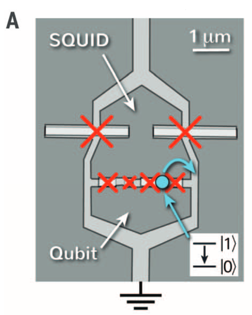

 , the average number of quasiparticles is represented by
  ,
,  is the relaxation time provided by a single quasiparticle, and
  is the decay of the qubit excitation into all channels. By fitting experimental data to Eq. 1, the authors are able to extract the quasiparticle number as a fit parameter, as well as distinguish the difference between qubit decays into quasiparticles versus decays into other channels. A measurement of the qubit lifetime and fit to Eqn. 1 is shown in Fig. 2. The authors find that the average quasiparticle number in this measurement is
  , the decay induced by a single quasiparticle is
  , and decay to all other channels is given by
  .
.
 , where
  is the resonant frequency of the qubit. In turn, the bath of quasiparticles must gain the same amount of energy,
  between
  (see. Fig. 2). By applying many of these pulses and continuously monitoring the qubit population, the authors see that the decay of the qubit excited state slows down with each consecutive
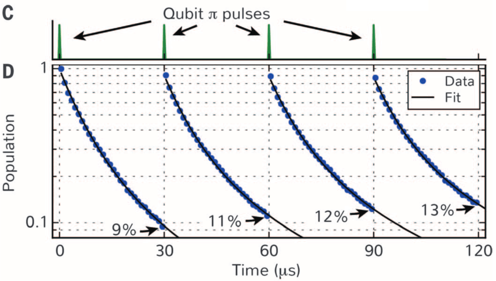
 between pumping pulses. After the last pulse, the authors measure the probability of the qubit being in its excited state as a function of time after the last pulse (a similar measurement to that in Fig. 3, only this time with the sequence of pumping pulses added to the beginning of the measurement protocol). The authors find that the qubit decay time increases with the number of pumping pulses, implying that each pulse is actually pushing these quasiparticles away from the qubit. The results are shown in in Fig. 4.
 T
T  s, finally the qubit is excited into its excited state and its decay is measured. (b) Results of the measured qubit decay as a function of the number of pump pulses. The observed qubit decay time increases with increasing pulse number. (c) The measured quasiparticle population, which is shown to initially decrease with pulses number before saturating near
  . (d) Measured induced decay per quasiparticle.
 . The authors also find that the lifetime of the qubit due to a single quasiparticle decreases with pulse number, which is somewhat surprising, since we would expect that each individual quasiparticle would impact the qubit lifetime in the same way. This feature is understood because as the number of pulses is increased, the quasiparticles near the qubit generally have larger energy and will actually give some energy back to the qubit as well as taking energy away from it. These competing factors may actually lead to a reduction of
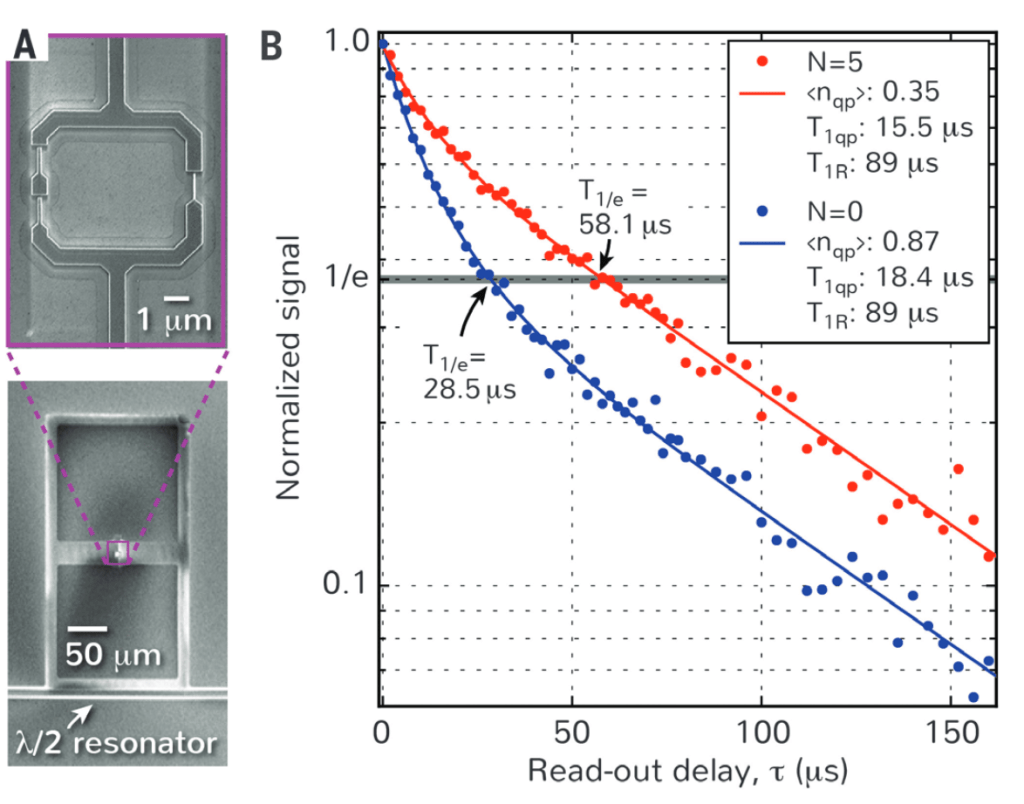

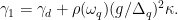
 es la tasa de decaimiento medida del cúbit,
  es el ancho de banda de la cavidad de microondas,
  es la fuerza de acoplamiento entre el cúbit y la cavidad,
  es la diferencia en frecuencia de resonancia entre el cúbit y la cavidad,
  es la densidad de estados del cristal fotónico a la frecuencia del cúbit, y
  representa el decaimiento del cúbit en canales de disipación aparte del cristal fotónico. Midiendo la tasa de decaimiento total del cúbit para varios valores de
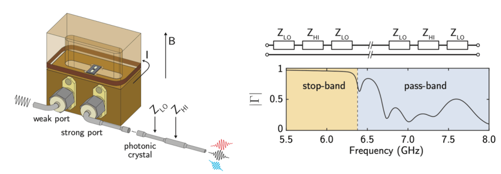
 que es desintonizado de la energía del cúbit una cantidad
  , donde
  es la frecuencia del impulso y
  , donde
  se conoce como frecuencia de Rabi generalizada. Este espectro de emisión se llama triplete de Mollow [2]. Ver Fig. 3 para un esquema de emisión del triplete de Mollow.
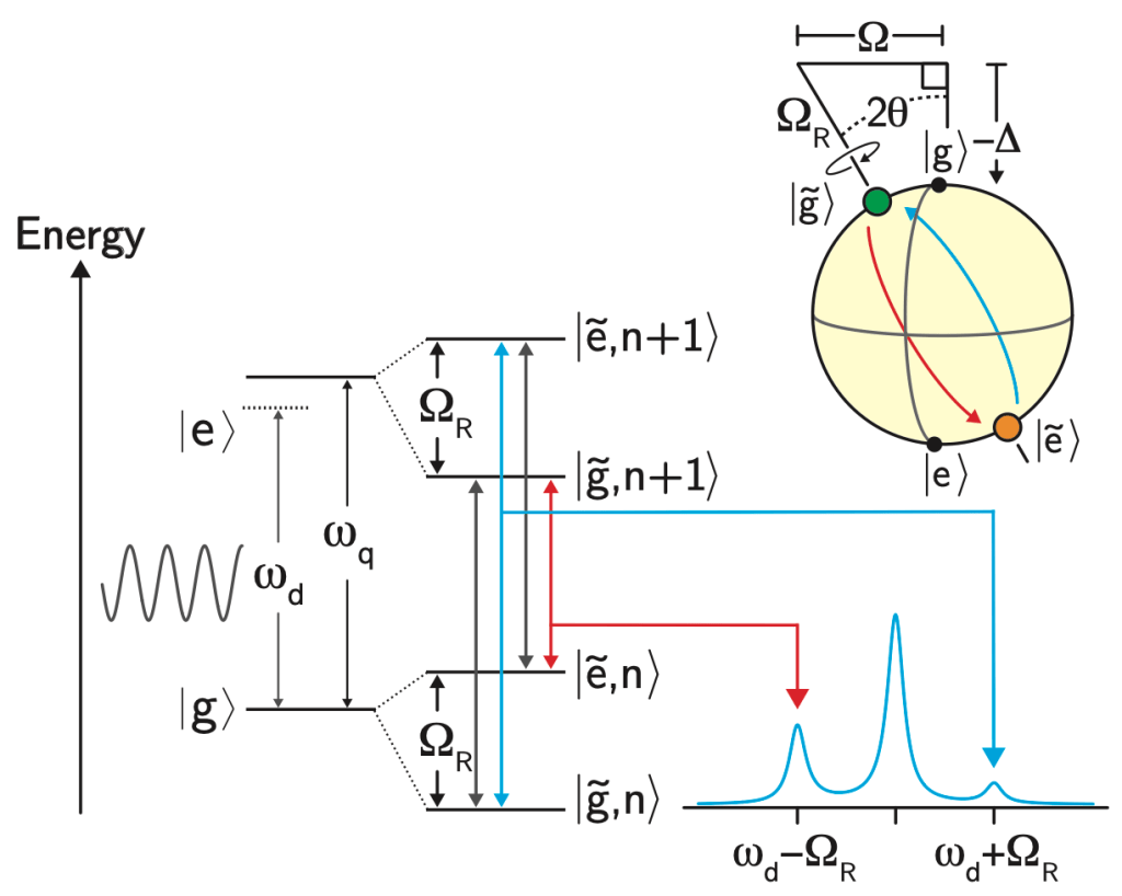
 . Debido al espectro de pérdidas modificado, el área de una banda lateral puede disminuir, indicando que el cúbit emitirá radiación a esta frecuencia en menor medida que la otra banda lateral. Arriba a la derecha: bajo la presencia del impulso, el eje de cuantización del cúbit también rota, lo cual cambia los estados del cúbit que se pueden preparar / estabilizar.
  , es posible que una de las bandas laterales del triplete de Mollow experimente una tasa de pérdidas grande mientras que la otra banda lateral experimenta una tasa baja.
 y
y  son matrices de Pauli. Dado que este hamiltoniano no es diagonal, es conveniente rotar la base de manera que el hamiltoniano se pueda escribir de la forma
 y el ángulo de rotación se define como
  con
con  . Dado que hemos escrito el hamiltoniano en una base rotada, debemos considerar también cómo rotan los nuevos autoestados del sistema con respecto a los autoestados originales, que llamaremos
  y
y  para los estados fundamental y excitado, respectivamente.
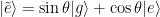
 , que inmediatamente nos informa de que
  , por lo que podemos reescribir los autoestados rotados del sistema como
 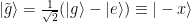 y
y  , los cuales tienen la propiedad especial de que
  . Dado que el estado
  tiene una energía menor, emitirá energía correspondiente a la banda lateral de menor energía del triplete de Mollow y viceversa para el estado
  . Si la pérdida del cúbit es muy diferente para cualquiera de estos estados, ¡fomentará el decaimiento hacia los estados
  tenderá a +1 en este supuesto! En el caso de un espectro de pérdidas uniforme, no habría un decaimiento preferido para el cúbit y sería de esperar que todos los valores esperados decayeran a cero.
![\dot{\rho} = i[\rho,H] + \gamma_0 \cos{(\theta)}\sin{(\theta)}\mathcal{D}[\tilde{\sigma}_z]\rho + \gamma_{-} \sin{^4\left(\theta\right)} \mathcal{D}[\tilde{\sigma}_{+}\rho + \gamma_{+}\cos{^4\left(\theta\right)} \mathcal{D}[\tilde{\sigma}_{-}]\rho.](https://s0.wp.com/latex.php?latex=%5Cdot%7B%5Crho%7D+%3D+i%5B%5Crho%2CH%5D+%2B+%5Cgamma_0+%5Ccos%7B%28%5Ctheta%29%7D%5Csin%7B%28%5Ctheta%29%7D%5Cmathcal%7BD%7D%5B%5Ctilde%7B%5Csigma%7D_z%5D%5Crho+%2B+%5Cgamma_%7B-%7D+%5Csin%7B%5E4%5Cleft%28%5Ctheta%5Cright%29%7D+%5Cmathcal%7BD%7D%5B%5Ctilde%7B%5Csigma%7D_%7B%2B%7D%5Crho+%2B+%5Cgamma_%7B%2B%7D%5Ccos%7B%5E4%5Cleft%28%5Ctheta%5Cright%29%7D+%5Cmathcal%7BD%7D%5B%5Ctilde%7B%5Csigma%7D_%7B-%7D%5D%5Crho.&bg=ffffff&fg=010101&s=0&c=20201002)
 es la matriz de densidad reducida para el cúbit, el superoperador de disipación también se introduce como
 ![\mathcal{D}[A]\rho = \left( 2 A \rho A^{\dagger} - A^{\dagger}A\rho - \rho A^{\dagger}A\right)/2](https://s0.wp.com/latex.php?latex=%5Cmathcal%7BD%7D%5BA%5D%5Crho+%3D+%5Cleft%28+2+A+%5Crho+A%5E%7B%5Cdagger%7D+-+A%5E%7B%5Cdagger%7DA%5Crho+-+%5Crho+A%5E%7B%5Cdagger%7DA%5Cright%29%2F2&bg=ffffff&fg=010101&s=0&c=20201002) . La tasa
. La tasa  representa un desfase del cúbit en la base rotada de
  y las transiciones entre autoestados en la base rotada son controlados por los operadores de “salto”
  , que están relacionados con las tasas
  . Similar al ejemplo anterior, si el cristal fotónico modifica la pérdida del cúbit tal que
  , el autoestado del sistema de referencia en rotación correspondiente se estabilizará.
 (¡que es mucho más largo que el tiempo de coherencia del cúbit en ausencia del impulso!). Durante este tiempo, el cúbit debería decaer preferiblemente a un autoestado del sistema rotado si las bandas laterales del triplete de Mollow tienen pesos diferentes. Una vez se corta el impulso, se mide el valor esperado
 ).
).  and isolated from everything else. For a given temperature, we know that the probability that the system is in a state with energy
  is given by
 is the well-known partition function, which roughly tells us how many different ways one can partition a system into subsystems having the same energy, and
  is the Boltzmann constant which relates absolute temperature to the kinetic energy of each microscopic particle in any given system.
  described by a Hilbert space
  which is decomposed into a system
  with Hilbert space
  and an environment
  with Hilbert space
  . In principle
  , but we can consider restrictions over the space as shown in the picture below.
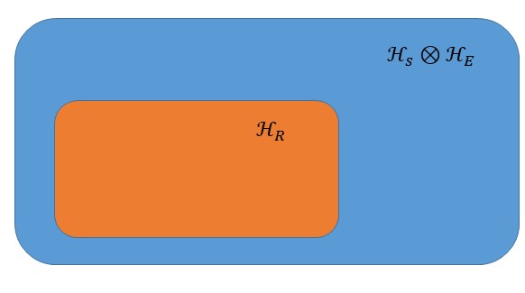
 smaller and would be analogous to the system presented in the introduction with a fixed temperature
  . In a quantum setting, such restrictions are described by considering constraints on the possible joint states of system
  , assuming that
  . If we had taken the system
  would correspond to the Gibbs state, which describes an equilibrium probability distribution that remains invariant under any future evolution of the system, with the probabilities given in the introduction. So far, we have just rewritten everything in the language of quantum mechanics but the authors take a step further. It’s important to remark that we could have taken any other restriction for
  and defines the state of the system
 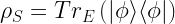 , then the authors show that
  is close to the state
  .
. .
.
 be the state obtained by tracing out the environment and define the set of states at a distance of the canonical state equal or greater to
  as
as  . The radius defined by
  is shown below.
 is a set in the Hilbert space
  (different from the one pictured above, which is the space of density matrices). We picture below the set
 of the canonical state as
 refers to the “volume” of the set in the argument. Another way of interpreting this ration is as the probability of picking a random state
  such that the distance of
  we have that
 and
and  .
.  grows, the probability, of picking a state such that the distance is big enough, decays exponentially.
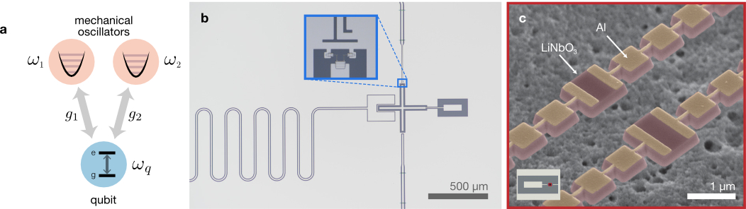
 con materiales superconductores. El elemento clave de este circuito es la unión de Josephson, que está hecha de óxido de aluminio intercalado entre capas de aluminio superconductor. La unión actúa como un inductor no lineal que modifica la distancia entre los niveles de energía del oscilador
  ) y el excitado (
 ). Los dos niveles forman un bit cuántico (cúbit). El cúbit está diseñado para que se pueda ajustar su frecuencia poniendo dos uniones de Josephson en paralelo. Aplicando un campo magnético mediante un cable que lleve corriente, se produce un flujo magnético a través de la espira que permite cambiar la frecuencia del cúbit.
 . Para acoplar el cúbit con los osciladores mecánicos, los autores usan la piezoelectricidad de la lámina de niobato de litio. El movimiento mecánico de este material produce una acumulación de carga eléctrica sobre los paneles de aluminio situados en ambos chips, que están diseñados para ser el elemento capacitivo del cúbit. El cúbit capacitor se carga con el movimiento de los osciladores mecánicos, garantizando que los dos sistemas están conectados.
  ). Nótese que las frecuencias mecánicas de los dos osciladores son diferentes, así que el cúbit sólo puede estar en resonancia con una a la vez. Esto permite el intercambio directo de energía entre el cúbit y cada oscilador a una tasa relacionada con el acoplamiento capacitivo entre los dos,
  9.5 MHz,
  10.5 MHz. El hamiltoniano que describe la interacción entre el cúbit y el oscilador mecánico en resonancia es la interacción de Jaynes-Cummings:
 y
y  son los operadores creación y destrucción para el oscilador mecánico y el cúbit, respectivamente. Cuando están en resonancia, el cúbit y el oscilador mecánico intercambian sus respectivos estados en un tiempo de
  24-26
24-26  dependiendo del oscilador en cuestión.
 y
y  , donde
  representa el estado de la mecánica y del cúbit. Entre un intercambio completo, el cúbit y los osciladores mecánicos están entrelazados con función de estado
  .
. o
o  . El estado
  describe el número de fonones de un oscilador mecánico concreto,
  …, y si el cúbit está en su estado fundamental o excitado
  . La frecuencia del cúbit se sintoniza para que esté en resonancia con alguno de los modos mecánicos durante el tiempo correspondiente a un intercambio completo. Cuando la operación de intercambio es aplicada al estado
  , el sistema permanece inalterado dado que ambos subsistemas están en su estado fundamental y no hay energía que intercambiar. Durante el intercambio, el estado
  . El oscilador mecánico está ahora en un estado de superposición, pero el estado del oscilador mecánico no está entrelazado con el estado del cúbit.
 , se determina ahora por el acoplamiento capacitivo directo,
  , la desintonización entre el cúbit y la mecánica,
  ), la interacción mostrada en la
 es la versión en operadores del número de fonones,
  , donde
  . Comparando el hamiltoniano combinado con el de sólo el cúbit, vemos que el efecto de la interacción es modificar la frecuencia de transición del cúbit (representado por todo lo anterior a
  ). Por cada fonón adicional en el oscilador mecánico, la frecuencia de transición del cúbit cambia
  y se deja precesar por un tiempo variable,
  . Durante este tiempo, el estado superpuesto acumula una fase de
  para dos fonones y así sucesivamente. La fase acumulada refleja la probabilidad (
 ) de que el oscilador mecánico contenga cero, uno, dos, etc. fonones. El estado del cúbit evoluciona a
  , donde la fase acumulada es
 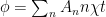 . Los autores rotan el cúbit de vuelta a su base de medición y monitorizan la población final del estado excitado como función del tiempo de interacción,
 ![S(t) = \sum_n A_n e^{-\kappa t/2} \cos [(2 n \chi t) + \phi_n]](https://s0.wp.com/latex.php?latex=S%28t%29+%3D+%5Csum_n+A_n+e%5E%7B-%5Ckappa+t%2F2%7D+%5Ccos+%5B%282+n+%5Cchi+t%29+%2B+%5Cphi_n%5D&bg=ffffff&fg=010101&s=0&c=20201002)
 . También incluye el desfase dependiente del número,
  y la constante de decaimiento de fonones,
  . Esto captura la dinámica de la trayectoria del cúbit incluso cuando las probabilidades de los fonones van cambiando debido al decaimiento de la energía. La figura a continuación muestra una traza de interferometría y el ajuste que se usó para extraer la población de fonones en el oscilador mecánico. La traza contiene una combinación de varias oscilaciones de frecuencia, cada una de ellas correspondiente a un número de fonones distinto. El peso de una frecuencia particular en la combinación representa la probabilidad de que el correspondiente número de fonones esté presente en el estado mecánico que se vaya a medir.
 , donde el oscilador mecánico contiene
  fonones y el cúbit puede estar tanto en el estado fundamental (
 ). Primero, se prepara el cúbit en su estado excitado con
  . Medio intercambio entre el cúbit y el primer oscilador mecánico los entrelaza,
  . Esto se consigue llevando el cúbit a resonancia con el oscilador mecánico sólo durante la mitad del tiempo requerido para llevar a cabo un intercambio completo, como se puede ver en la
  . Esto deja al cúbit en su estado fundamental con los dos osciladores mecánicos completamente entrelazados entre sí
  .
.