Authors: Hsin-Yuan Huang, Richard Kueng, John Preskill
First Author’s Institution: California Institute of Technology
Status: Pre-print on arXiv
In the past few years, machine learning has proven to be an extremely useful computational tool in a variety of disciplines. Examples include natural language processing, image recognition, beating players at Go, quantum error correction, and shifting through massive quantities of data at CERN. As is often the case, we may choose to ponder whether replacing classical algorithms by their quantum counterparts will yield computational advantages.
The authors consider the complexity of training classical machine learning (CML) and quantum machine learning (QML) algorithms on the class of problems that map a classical input (bit string) to a real number output through any physical process (including quantum processes). The goal of the ML algorithms is to learn functions of the following form: . Unpacking the notation, we see that given some input bit string that designates an initial quantum pure state, we get an output by processing the input through a quantum channel and then determining the expectation value of an operator with respect to the output of the channel (i.e. quantum evolution of the initial state). The ML algorithms will attempt to predict the expectation value of after training on many input bit strings and channel uses. You may wonder whether a single bit string is a sufficiently complicated input, but recall that all of the movies you watch, the articles on Wikipedia you read, and the music you play on your computer are represented by bit strings. Given a sufficiently long input bit string, we can feed into our algorithm arbitrarily long and precise classical data. What is very interesting about this class of problems is that we can describe quantum experiments with many different input parameters in this language, meaning the ML algorithms are being trained to predict the outcome of (potentially very complicated) quantum physical experiments. This could include predicting the outcome of quantum chemistry experiments, determining the ground state energy of a system, or predicting a variety of other observables from a myriad of physical processes.
As is often the case, there isn’t a single clear answer to the question posed, but the authors discuss two scenarios of interest. First, a secnario in which QML models pose no significant advantage over CML models and another in which QML models provide exponential speedup. According to the paper, if one consider’s minimizing average prediction error (over a distribution of all the inputs), then QML doesnotprovide a significant advantage over classical machine learning. However, if one is interested in minimizing worst-case prediction error (on the single input with the worst error), then quantum machine learning requires exponentially fewer runs of the quantum channel.
What are the ML Models of Interest?
The goal of supervised machine learning is to use a large quantity of input data and a corresponding set of outputs to train a machine to generate accurate predictions from new data. In this paper, the objective is to see how many times it is necessary to run a physical process such that the machine can accurately predict the results of the experiments to some tolerance. The scaling of the number of times the quantum process is used in the training phase of the algorithm defines the complexity of the algorithm. Each of the ML algorithms generates a predictive function , where the prediction error on each input is given by . If given a probability distribution over all possible inputs, we would like to figure out the number of times that must be run to either produce an average-case prediction error of or a worst-case prediction error given by .
The quantum advantage arises only when one considers the worst-case prediction error instead of the average prediction error.
It is very reasonable to think quantum machine learning would be better than classical machine learning when trying to predict the outputs of quantum experiments, but the main result throws that assumption into question. We begin by explaining how QML and CML are defined.
Figure 1: Illustration of classical and quantum machine learning models (Figure 1 from article)
Classical ML models are composed of a training phase that consists of taking a randomized set of inputs and performing quantum experiments defined by a physical map (a CPTP map) from a Hilbert space of qubits to one of qubits that yields an output quantum state for each input. However, CML needs to be trained on classical output and so a POVM measurement (which is a generalization of a projective measurement) is performed that yields an output . Any classical machine learning algorithm (neural networks, kernel methods, etc.) can then be applied to generate the predictive function that approximates (the true function) from the set of pairs of inputs and classic outputs . Here denotes the number of times that applying the channel is required for CML since it is only possible to obtain one input/output pair per channel usage. The authors present a further restricted classical ML algorithm, which is identical to the general case, but where instead of doing arbitrary measurements to generate the outputs, only the target observable is directly measured.
A quantum ML model has the same goal as the classical models, but has the added advantage that the algorithm can be trained directly on quantum data. The general flow is that given an initial state on many qubits, the quantum channel is applied times with quantum processing maps inserted in between applications. The quantum data processing maps take the place of the classical machine learning algorithms. The resultant state that is stored in quantum memory is the learned prediction model. To predict new results, the final state after all of the channel applications and processing () is measured differently based on the desired input bit strings . The outcomes of these measurements are the outputs of the predictive function that approximate the desired function .
The Meat of the Paper
Average-case Prediction Error Result
The main results of the paper are presented in the form of theorems. The first theorem shows that if there exists a QML algorithm with an average prediction error bounded by that requires uses of the channel , then there exists a restricted CML algorithm with order average prediction error that requires channel uses. The training complexity of the classical algorithm is directly proportional to that of the quantum model up to a factor of where is the number of qubits at the output of the map .
Sketch of First Theorem Proof
Consider an entire family of maps that contains the map of interest. Cover the space of the family of maps with a net by choosing the largest subset of maps such that the functions generated by different maps are sufficiently distinguishable over the distribution of inputs . (In the paper they take the average-case error between any two different elements of to be at least ).
The proof proceeds as a communication protocol that starts by having Alice choose a random element of the packing net (). Alice then prepares the final quantum state by using the chosen channel times and interleaving those uses with the quantum data processing maps . This results in the state the QML algorithm is supposed to generate to make predictions through measurements. Alice then sends to Bob and hopes he can determine what element of the packing net she initially chose by using the predictions of the QML model. Bob can then generate the function that approximates with low average-case prediction error by construction. Moreover, because the different elements of the packing net are guaranteed to be far enough apart, Bob can with high-probability determine which element Alice chose. Assuming Bob could perfectly decode which element Alice sent, Alice could transmit bits to Bob. With this scheme we expect the mutual information (a measure of the amount of information that one variable can tell you about another) between Alice’s selection and Bob’s decoding to be on the order of bits. The authors now make use of Holevo’s theorem, which provides an upper bound on the amount of information Bob is able to obtain about Alice’s selection by doing measurements on the state . This is on the order of the previously given mutual information, however, it is also possible to relate the Holevo quantity directly to the number of channel uses required to prepare the state Bob receives. Through an induction argument in the Appendix, the authors show the Holevo information is upper bounded by . From this it follows that the number of channel uses for the quantum ML algorithm is lower-bounded by .
All that’s left is to relate the number of channel uses required for the QML model to the necessary number needed for the classical machine learning algorithm. A restricted CML is constructed such that random elements are sampled from and the desired observable is measured after preparing each time. As mentioned earlier, experiments are performed. The pairs of data are used to perform a least-squares fit to the different functions of the packing net, which are sufficiently distinguishable as defined earlier. Therefore, given a sufficiently large number of data points, it is possible to determine which element of the packing net was used as the physical map from the larger family of maps. The authors show that if the number of points obtained is on the order of , it is possible to find a function that achieves an average-caseprediction error on the order of . Relating and through directly yields that . Hence, if there is a QML model that can approximately learn ,then there is also a restricted CML model that can approximately learn with a similar number of channel uses. This means that there is no quantum advantage in terms of the training complexity when considering minimum average-case prediction error as any QML model could be replaced by a restricted CML model that achieves comparable results.
Worst-case Prediction Error Result
The second main result states that if we instead consider worst-case prediction error, then an exponential separation appears between the number of channel uses necessary in the QML and CML cases. This is shown in the paper through the example of trying to predict the expectation values of different Pauli operators for an unknown -qubit state. As a refresher, the Pauli operators () are 2×2 unitary matrices that form a basis for Hermitian operators, which correspond to observable operators in quantum mechanics. Since any Hermitian operator can be decomposed in terms of sums of Paulis, it is natural to wonder about the different expectation values of each Pauli operator given an unknown state. Given a -input bit string we can specify an -qubit Pauli operator and the channel , which both generates the unknown state of interest and maps to a fixed observable . Therefore, the function we are getting the ML model to learn is . The authors show that by cleverly breaking the QML model into two stages, the first of which is estimating the magnitude of the expectation value () and the second estimating the sign of the expectation value, only channel uses are necessary to predict expectation values of any Pauli observables. Therefore it is possible to predict all Pauli expectation values up to a constant error with only a linear scaling in the number of qubits (). On the other hand, the paper shows the lower bound for estimating all the expectation values of the Pauli observables using classical machine learning is . Therefore, there is an exponential separation between QML and CML models in the number of channel uses necessary for predicting all Pauli observablesin the worst-case prediction error scenario. The authors numerically demonstrate the difference in complexity between the different types of algorithms and show the separation clearly exists for a class of mixed states, but vanishes for a class of product states.
Takeaways
Classical machine learning is much more powerful than may be naively assumed. For average-case prediction error, CML models are capable of achieving a comparable training complexity to QML models. This means we may not need not to wait for QML to predict the outcomes of physical experiments. Performing quantum experiments and using the output measurements to train CML models is a process that can be implemented in the near-term. In the case of approximately learning functions it appears that using a fully quantum model does not provide a significant advantage. However, the authors did demonstrate an interesting class of problems in which QML models are capable of exponentially outperforming even the best possible classical algorithm. The question is whether there are interesting tasks that require having a minimum worst-case prediction error, where learning the function over a majority of inputs does not suffice. I leave it to the reader as an exercise to search out other interesting learning tasks where quantum advantage is achieved and where the classical world of computing does not suffice.
Ariel Shlosberg is a PhD student in Physics at the University of Colorado/JILA. Ariel’s research focuses on quantum error correction and finding quantum communication boundsand protocols.
Title: Universal non-adiabatic control of small-gap superconducting qubits
Authors: Daniel L Campbell, Yun-Pil Shim, Bharath Kannan, Roni Winik, David K. Kim, Alexander Melville, Bethany M. Niedzielski, Jonilyn L. Yoder, Charles Tahan, Simon Gustavsson, and William D. Oliver
Are two qubits better than one? In this QuByte, we will be looking at a new variation of superconducting qubits, proposed by the EQuS lab at MIT. The new qubit, referred as a superconducting composite qubit (CQB), is made up of two coupledtransmon qubits. The authors of the paper answered the question in the affirmative: the composite qubit is more resilient to environmental noise permitting a longer qubit lifetime than a single transmon qubit. Moreover, the fast and high-fidelity gate operations in the composite qubit utilizing Landau-Zener interference require less microwave resources compared with standard on-resonance Rabi drive techniques. In this QuByte, we review the mechanism of Landau-Zener (LZ) interference, and elucidate its role in qubit state initialization and gate implementation.
The composite qubit itself
Optical image of two composite qubits, () is the reduced magnetic flux that determines the frequency of each transmon, controlled in real time by the arbitrary waveform generators (AWGs); and are the microwave control fields for qubit state readout and initialization, respectively.
The composite qubit is formed by two transmons capacitively coupled together. When using a single transmon as a qubit, its energy eigenstates are used to encode information so that and where denotes the transmon index. A single transmon qubit has frequency –that is, the energy difference between its ground state and the excited state . This frequency is controlled by the magnetic flux threading the SQUID loop of the transmon circuit. In the figure below, the dashed lines show the transmon frequency as a function of the reduced magnetic flux where is the magnetic flux quantum. As two transmons are flux-tuned to and they should have the same frequency . But instead of their energy levels crossing an energy gap called an “avoided crossing”appears for the coupled transmons (solid lines in the plot below). The magnitude of the avoided crossing is 65 MHz in this device, and it depends on the coupling strength between two transmons. (For an intuitive and pictorial explanation of avoided crossings, I recommend this wonderful article with a classical example of coupled mechanical oscillators.)
Qubit energy spectrum as a function of the flux biases; dashed lines: frequencies of bare transmon states (diabatic states); solid lines: frequencies of the coupled two-transmon states (adiabatic states). The avoided crossing of size 65 MHz appears at when two transmons are biased at the same frequency .
At the avoided crossing, the eigenstates of the system are the equal superposition states of bare transmon states which we use to define a computational basis of a qubit: . By this definition, the composite qubit has the frequency of the gap =65 MHz.
The composite qubit device emulates the following qubit Hamiltonian: , with states and associated with the eigenstates of , and the bare transmon states and associated with the eigenstates of . The parameter in the second term is determined by the frequency difference between the two bare transmons , and is controlled by varying the flux biases on the individual transmons simultaneously as a function of time. As we expect, at the composite qubit operating point , the qubit exhibits an energy splitting of .
Landau-Zener interference
To understand how gates are implemented in this new qubit, we must first understand Landau-Zener interference. For a system described by the aforementioned Hamiltonian , let’s denote its instantaneous eigenstates as and , corresponding to the lower and the higher energy eigenstates, respectively. The adiabatic theorem tells us that if the qubit state is initialized in one of the eigenstates, say , and if the time-dependent term in the Hamiltonian changes infinitely slowly, then the qubit always remains in that eigenstate throughout the evolution. However, If is varied such that the system traverses the avoided level crossing region in a finite time, a transition between two energy levels can occur and the final state becomes a linear combination of two instantaneous eigenstates. This transition between two energy levels that takes place while traversing the avoided crossing is called the Landau-Zener transition. It acts as a coherent beam splitter for a qubit state. The transition probability from state to is defined and depends on the size of the avoided crossing as well as the “velocity” of traversing the avoided crossing region . (For a pedagogical derivation of this formula, see Vutha). Moreover, if the is varied periodically such that the system traverses the avoided crossing multiple times, a sequence of LZ transitions can be induced. The phase accumulated between successive LZ transitions can constructively and destructively interfere in a controlled manner, which can be used to create a general superposition state.
In the following, we will see, the adiabatic evolution (i.e. varying slowly) is used for state initialization. The non-adiabatic LZ transitions induced by quickly varying at the avoided crossing are used to implement gates to modify quantum states.
Qubit state initialization
To use the composite qubit to encode information, one needs to be able to initialize it into the computational states or . The state initialization protocol makes use of adiabatic evolution: we vary the system ( in this case) very slowly such that if the system starts in an eigenstate of the initial Hamiltonian, it ends in the corresponding eigenstate of the final Hamiltonian. Let’s go through it step by step, and it will become clear exactly how slow the change in needs to be.
Energy levels of transmons 1 and 2 in the presence of a coherent microwave field with frequency and amplitude .
Start with both transmons in their ground states (corresponds to the filled in black circle in the figure above). This is achieved by waiting a sufficient time for the transmons reach the thermal equilibrium as the transmon temperature (around 40 mK at the bottom of the dilution fridge) is much smaller than their energy gaps (around 7 GHz for both transmons) so that and the transmon thermal state is approximately its ground state. Then turn on a static coherent microwave drive field of frequency ; this drive hybridizes the states and as shown in the diagram above, and causes a splitting with magnitude in the qubit energy spectrum. This splitting is known as the Autler-Townes splitting, and describes how the energy spectrum of an atom is modified when an oscillating electric field is close to resonance with the atom transition frequency.
Sweep the frequency of transmon 2 by tuning its flux bias . Let be the detuning between transmon 2 frequency and the drive frequency , and sweep through the drive frequency slowly such that the transmon state adiabatically evolves to (to the filled in purple circle in the figure above). The final occupation probability of state (i.e., the probability of remaining in the upper energy level during the sweep) is given by one minus the Landau-Zener transition probability . Thus we see that high-fidelity state initialization requires that the change in transmon 2 frequency be slow enough such that .
Turn off the drive, adiabatically tune the transmons in fluxes to the composite qubit operating point so that the qubit state adiabatically evolves to .
Similarly, one can prepare the logical state by adiabatically evolve the state: . It takes about 250 ns to complete the above state initialization steps; this is mostly limited by how slow the change of the system needs to be to meet the adiabatic condition .
Single-qubit gates
In the following, we will talk about some elementary gates that are used to manipulate the state of a single composite qubit, namely, the X, Y and Z gates. The X and Y gates change the probabilities of measuring the qubit in a state or , whereas the Z gate modifies the relative phase between states and . Their operations can be visualized in the Bloch sphere representation as rotations of the qubit state around the -, – and -axes, respectively. In composite qubits, the single-qubit gates are implemented through the transmon flux controls . The physical set-up involves using arbitrary waveform generators (AWGs) to generate electrical current waveforms in the transmon circuits. This in turn leads to the time-dependent magnetic fluxes to control the transmon frequency difference as desired.
-gates
The flux control pulse to implement Z gates, .
A -gate implements a rotation around -axis in the Bloch sphere representation of qubit states. This rotation is described by a unitary operator, parameterized by a rotation angle : . The Z-gate of the composite qubit is realized by simply idling the qubit (that is, biasing the qubit with a constant magnetic flux) at the avoided crossing , as shown in the schematic above, and letting the qubit evolve under the Hamiltonian for some gate time . Governed by the Schrodinger equation, the evolution of the state from the initial state to the final state after applying Z-gate is given by an unitary operator , i.e., , where – this is exactly the unitary we need to realize a -gate; the gate time controls the rotation angle .
and gates
In transmon qubits, X and Y gates are conventionally implemented by subjecting a qubit to a continuous microwave driving field on resonance with the qubit. If the qubit has non-degenerate energy levels, under this drive, the probability amplitudes of the qubit state on its ground and excited states oscillate – this oscillation is referred as the Rabi oscillation. For a transmon qubit with a frequency of a couple of gigahertz, the gate time of this type is on the order of tens of nanosecond. How fast and how accurately these gates can be implemented are restricted by the validity of the rotating wave approximation. This approximation allows one to neglect the fast-oscillating terms in treating and describing Rabi oscillations, and it only holds true for qubits with large transition frequencies. For a composite qubit with a small gap on the order of tens of MHz between between its computational states, the Rabi drive will be complicated to deal with, both mathematically and practically, due to the breakdown of this approximation. The alternative solution here, as you may have already guessed, is to use LZ transitions in small-gap qubits to manipulate qubit states.
Take the single-qubit gate as an example; in the Bloch sphere representation, this gate rotates the qubit state about the -axis by an angle . The schematic below shows the control for its implementation. This protocol is designed to induce non-adiabatic LZ transitions at the avoided crossings to manipulate the qubit’s state. Specifically, the control pulse contains a period of sinusoid pulse with idling operations (i.e., constant flux biases at the avoided crossing, equivalent to Z-gates) padded before and afterwards.
The flux control pulse to implement X gates
During the implementation of the gate, the flux controls on two coupled transmons are varied simultaneously with respect to the avoided crossing. Let denotes how much the flux controls are biased away from the avoided crossing bias point (i.e., and ), let be the instantaneous eigenstates of the time-dependent Hamiltonian so that , and let be the energy gap between two states. The plot below shows how the qubit energy gap changes with respect to the flux detuning , which is varied in time as shown in the lower panel of the plot.
Upper: the measured CQB excited state spectroscopy to form a two-level system; lower: non-adiabatic control implemented by a non resonant sinusoidal excursion about the avoided crossing.
The dashed lines in the lower panel marked at 1, 2 and 3 correspond to the start, the middle and the end of the sinusoidal flux tuning. Here is a glance of what happens to the qubit state during this sinusoidal excursion about the avoided crossing :
At () an LZ transition takes place as the qubit state leaves the avoided crossing.
During () phase accumulates between the two qubit eigenstates.
At () another LZ transition takes place when the qubit traverses the avoided crossing.
During () phase accumulates between the qubit eigenstates (the same as what happened during ).
At () another LZ transition takes place when the qubit returns to the avoided crossing.
To better illustrate this process, let’s redraw the previous plot of the qubit energy levels during the sinusoid pulse as a function of time:
A sketch of the time-dependent qubit energy levels during the sinusoidal flux pulse.
The non-adiabatic LZ transitions induced at the time points 1, 2 and 3 are described by a unitary operator . Thus, the occupation amplitude in the upper and lower eigenstates interfere, resulting in the state transitions with the probability , and a relative phase introduced between and .
During the adiabatic evolution from time 1 to 2 and from time 2 to 3, the upper energy state acquires a phase relative to the lower energy level ; no LZ transition is encountered due to adiabaticity. For the evolution , the phase accumulated is . Geometrically this can be interpreted as the area under the curve (the shaded yellow area above). Similarly, for the evolution the accumulated phase is (the shaded blue area above).
The process described above is, in effect, an interferometer made out of beam splitters placed at the avoided crossings; the fast changing fluxes near in the sinusoid induce transitions between the upper and lower energy branches just like how a beam splitter splits light into different optical paths. Similarly, the slow changing fluxes away from contribute to the phase evolution and set the stage for constructing and destructive interference between successive LZ transitions just like how sources of light creates interference pattern depending on their relative phase. The differences between the two scenarios are as follows: the optical interference is between photons, while here the interference is between quantum states of a superconducting qubit; the optical interference pattern is determined by the optical length, while here the interference happens in the phase space and is determined by the time-dependent qubit energy splitting; and lastly the qubit LZ interferometer is more fragile than an optical interferometer since photon states are very robust to decoherence.
As explained above, the evolution under the sinusoidal flux pulse can be seen as a combination of X-rotations (state transition) and Z-rotations (phase evolution). Padded Z-gates are introduced to cancel out the excess Z-rotation to implement a pure X gate with a desired rotation angle. The start of the pulse, once chosen, establishes an x-axis of the Bloch sphere. The gate, a rotation around y-axis, is then implemented by advancing the onset of the pulse by the time which corresponds the gate time of a gate, i.e., , as shown below.
The flux control pulse to implement Y gates
The frequency of the sinusoidal pulse realized by the flux controls is chosen to be = 125 MHz (corresponds to a 8 ns sine pulse). The frequency of the sine pulse (thus determines the gate time) is chosen such that the passage through the avoided crossing is fast enough to induce LZ transitions, but also not too fast so fast that successive LZ transitions overlap with each other. The flux control can be easily realized using an arbitrary waveform generator. Compared with the Rabi-type of gates where one needs to modulate the microwave signal at several gigahertz which require expensive microwave generators and IQ mixers, the type of gates here using LZ interference are simpler and cheaper to implement in the hardware.
Let’s overview how quantum computation would proceed using a composite qubit. It begins by initialization the qubit in the computational state or using the adiabatic evolution we described previously via a static microwave field. The single-qubit X and Y gates are implemented using LZ interference, and the Z gate is implemented by the idling operation. To complete a universal gate set for quantum computation, the two-qubit controlled-Z (CZ) gate is also demonstrated in the paper by turning on an effective interaction between two composite qubits. This interaction is realized by adiabatically tuning the frequency of the second composite qubit to realize an avoided crossing that evolves the second excited state of the bare transmons – this operation is similar to how a CZ gate is implemented between two standard transmon qubits. The composite qubit state is read out by uniquely mapping the computational states and to the bare transmon states and by the adiabatic evolution, and then read out through the readout resonators as in standard transom qubits.
Noise immunity
Finally, let me discuss why it is better to use two transmons instead of one as a qubit. Recall we choose the eigenstates of the coupled transmons at the avoided crossing as the qubit states and . Remarkably, this choice of computational basis allows immunity to certain noise process. For example, the processes of thermal excitation and energy relaxation (the former causes the transition and the latter ) are sources of errors in a single transmon qubit. However, to cause a transition between the qubit computational states and , it takes a correlated excitation and relaxation event to flip the states of both transmons. Flipping the states of both transmons is less likely to happen as it requires a correlated two-photon interaction with the environment; this makes the composite qubit states insensitive to uncorrelated state transitions in single transmons. As a figure of merit for qubit lifetime, the time measures the timescale on which state transition between qubit states occurs. The measured of a composite qubit is longer than 2 ms – this is 2 orders of magnitude longer than that of a single transmon. The relaxation process to the state , however, takes the qubit state out of the computation subspace – this happens on the timescale of tens of microseconds (comparable to the time of the bare transmons). The good news is that this leakage error can be detected by continuously monitoring the readout resonators when biased at the avoided crossing, since the leakage to state will result in a shift on the resonant frequency of the readout resonator; while errors of this sort can occur, they are easily detectable.
Furthermore, the composite qubit is robust to the frequency fluctuations in individual transmons; for example, in a single transmon qubit the frequency fluctuations due to environmental flux noise and the photon shot noise from the readout resonator cause the qubit to decohere. However, when biased at the avoided crossing, the qubit frequency of the composite qubit is determined by the fixed coupling strength between two transmons, and thus is insensitive to bare transmon frequency fluctuations. Another figure of merit for the qubit lifetime is the qubit decoherence time , which measures the time scale on which the qubit goes from a maximal superposition state to a classical probability mixture. The time of the composite qubit, measured in a Hahn echo decay experiment, is reported to be greater than 23 s which is much larger than the of 3 s for a single transmon qubit.
I hope now you are convinced that it is worthwhile to use two transmons as one qubit to gain protection against certain environmental noise. With the protected computation states come the new challenges in performing state initialization and state manipulate for qubits in low frequency regime. The authors of the paper demonstrate that it is feasible to use adiabatic evolution to initialize states in a qubit with frequency below the environmental temperature, and to use the Landau-Zener interference to perform fast qubit gates.
The solutions demonstrated here can be extended to other types of small-gap superconducting qubits with near-degenerate eigenstates. For instance, the gate operations using the Laudau-Zener interference has been implemented in the early pioneering works on superconducting charge qubits, more recently in fluxoniums, and may be found useful in some new qubit designs, for example, the 0- qubit, the very small logical qubit (VSLQ) design. The results of today’s paper highlight an inexpensive flux control protocol that performs universal control in small-gap superconducting qubits, paving the way to a more scalable hardware architecture as researchers push for larger qubit numbers.
Haimeng Zhang is a PhD student in Electrical Engineering at the University of Southern California. Haimeng’s research focuses on non-Markovian dynamics and quantum error suppression protocols in superconducting qubits.
Title: Quantum Computations with Cold Trapped Ions
Authors: Ignacio Cirac, Peter Zoller
Status: Published 1994 in Physical Review Letters
In 1994, theorists Ignacio Cirac and Peter Zoller published a paper that marked the birth of a new field in experimental physics: trapped-ion quantum computing.
The idea that we could use quantum systems to solve some problems more efficiently than classical computers had been around for a while already, but Cirac and Zoller proposed a key component to the physical realization of an actual quantum computer on a trapped-ion system: the two-qubit gate.
Trapped ions were a natural choice for quantum computers because the technology for controlling these systems at the quantum level was already advanced. Laser cooling, a staple technique in atomic physics, was first demonstrated on a cloud of ions, and quantum jumps were first observed in single trapped-ion systems.
So, when buzz about universal quantum computers began, the ion trappers tuned in. They thought they had (or could develop) all of the tools necessary to build the first quantum computer.
There are a few requirements for making a quantum computer, but two of the most fundamental are:
Good qubits with long coherence times relative to the calculation time. This means that:
If the qubit is in state it will remain so without decaying to state and vice versa. (In the field of quantum computing, the time it takes for this decay to happen is known as “T1 coherence time” or “energy coherence time.”)
If the system is in a superposition state then the phase relationship between the two terms will remained well defined, i.e. there is no “dephasing” noise. The time for an equal superposition state, , to completely dephase to an orthogonal state, , is known as “T2 coherence time” or “dephasing time.”
A way to implement multi-qubit gates. These are the basic building blocks of any computational algorithm. In classical computing this would be like an AND or an OR gate. The quantum version of these gates are a little more complex, however, since the outcome of these gates is often an entangled state among the qubits involved. But you need just one two-qubit gate combined with single-qubit rotations to build a universal quantum computer.
The first point is easy. We just have to define two states in the ion to be the qubit states and . As long as the upper state is long-lived and the qubit is sufficiently isolated from the environment, trapped-ion qubits can have extremely long coherence times (the record is over 10 minutes! [1]).
But point two wasn’t quite so obvious when people first started considering a trapped-ion quantum computer. You can’t directly couple the electronic levels of two different ions to share their quantum information, so they needed an indirect way to mediate coupling between two qubits. This ended up being the shared motion of the ions in a trap.
Let me explain. An ion confined in a harmonic trap will have its motional energy quantized into harmonic oscillator levels . If there are ions in this trap, then, just like coupled harmonic oscillators, the system is defined by the normal modes of motion shared among the ions in the trap. This means that, because the ions are electrically charged and thus through their Coulombic repulsion the motion of one ion affects the motion of another, we can use this interaction to couple qubits together—as an information bus for multi-qubit gates.
But this only works if we have a way to couple the qubit to the motion. In 1994, when this paper was written, this coupling had already been demonstrated. Through laser cooling, physicists showed that light could be used to control the motion of an atom [2]. And through an extension of the general laser cooling concept, physicists showed that they could use light to couple the electronic degree of freedom to a single, particular harmonic oscillator energy level, provided the transition linewidth is narrow enough that these harmonic levels can be resolved. This is known as a resolved sideband interaction [3].
If an ion is in state the ground qubit state and the nth motional energy level, , then we can drive this sideband transition by applying a laser whose frequency , where is qubit frequency splitting and is one of the shared motion normal mode frequencies. Depending on whether we choose a positive or negative detuning, this will cause a blue sideband transition up to or a red sideband transition to , respectively. In this way we can add and subtract single phonons from the trapped ion system, which can allow us to cool the system to the ground state of motion and also move information from the electronic state of one ion to the electronic state of another by transferring it through their shared motional mode.
One important thing to note: if we start in , then applying a red sideband will do nothing, since there is no motional energy level lower than , which is necessary to satisfy energy conservation in this case. The same reasoning can be applied for the case where we try to apply a blue sideband pulse on a starting state —there is no motional state below , so the blue sideband does nothing to this state. See the figure below for a pictorial representation:
So how do you make a two-qubit gate out of this interaction? Starting with ions with all modes cooled to the ground state of motion, and three relevant internal energy levels, , , and (where and are the qubit levels and is an auxiliary level) Cirac and Zoller proposed the following three steps:
Red sideband -pulse between and on ion 1. This will move the population in state to state and add a quantum of shared motion to the system. It will do nothing to state . (The subscript outside of the ket denotes which ion.)
Red sideband -pulse between and on ion 2. If a quantum of motion was added in step 1, then this will cause a transition between and . Since it is a -pulse, the population won’t change, but it will acquire a phase shift.
Red sideband -pulse between and on ion 1. This transfers anything in back to , leaving the system back in the ground state of motion.
Now, let’s look at a truth table of the results of these pulses on two qubits. From the original paper we get:
If we combine this gate with single qubit rotations (and reverting back to standard qubit state labels and ), then the truth table can be simplified to:
This is the controlled-NOT (CNOT) gate. The first ion acts as the “control” qubit. If it is in state , then a NOT gate is performed on the “target” qubit, or ion 2, which flips the state of the qubit. If the control qubit is , then nothing happens.
The fact that this proposal enabled quantum computing on trapped ions with such a simple series of pulses created a ton of excitement among ion trappers. However, it had one fatal flaw: if the ions’ motion heats up during the gate, then it will fail. Keeping ions in the ground motional state for long periods of time unfortunately was an unrealistic expectation, since their motion is extremely sensitive to electric field noise. So, while this is a very important paper from a historical perspective, the Cirac-Zoller gate is not used in any modern trapped-ion quantum computers. In fact, it was never experimentally realized with the originally proposed setup, since a few years after this proposal, Klaus Mølmer and Anders Sørenson came up with their scheme for a two-qubit gate that was more robust to ion heating [4]. The Mølmer-Sørenson gate is still commonly used today.
[1] Wang, Y., Um, M., Zhang, J. et al. Single-qubit quantum memory exceeding ten-minute coherence time. Nature Photon11, 646–650 (2017). https://doi.org/10.1038/s41566-017-0007-1
[2] D. J. Wineland, R. E. Drullinger, and F. L. Walls. Radiation-Pressure Cooling of Bound Resonant Absorbers. Phys. Rev. Lett. 40, 1639 (1978).
[3] Diedrich, F., Bergquist, J., et al. Laser cooling to the zero-point energy of motion. Phys Rev Lett.62:403-406 (1989).
[4] Sørensen, A., Mølmer, K. Quantum Computation with Ions in Thermal Motion. Phys. Rev. Lett. 82 (9): 1971–1974. (1999). arXiv:quant-ph/9810039
First Author’s Institution: University of Copenhagen
Status: Pre-print on arXiv
The Big Idea
The authors develop a theoretical technique to identify situations where a noisy quantum computer without error correction loses to current classical optimization methods. The authors use their technique to provide estimates for many popular quantum algorithms running on near-term devices, including variational quantum eigensolvers,quantum approximate optimization (both gate-based), and quantum annealing (think D-Wave). The authors found that for quantum computers without error correction “substantial quantum advantages are unlikely for optimization unless current noise rates are decreased by orders of magnitude or the topology of the problem matches that of the device. This is the case even if the number of qubits increases.”
The author’s conclusion allows others researchers to identify and focus on the slim regime of experiments where quantum advantage without error correction is still possible, and shift more time into development of error-corrected quantum computers. Even seemingly “negative” results advance the field in meaningful ways.
Currently in Quantum Computing
Current quantum computers are noisy (errors frequently occur), and of intermediate size: large enough to compete with the best classical computers on (almost) useless problems, but not large enough to be fault-tolerant (~50-100 qubits). A fault tolerant quantum computer has enough error correction so that errors mid-calculation do not affect the final result. Fault tolerance requires more and better qubits than are available today. The community is fairly confident fault tolerant quantum computers will outperform classical computers on many useful problems, but it is unclear if noisy, intermediate scale quantum (NISQ) computers can do the same.
Optimization problems are a very useful, profitable, and ubiquitous class of problem where the goal is to minimize or maximize something: cost, energy, path length, etc. Optimization problems occur everywhere, from financial portfolios to self-driving cars, and often belong to the NP complexity class, which is widely accepted as extremely difficult for classical computers to solve. Comparing computers based on ability to solve optimization problems has two benefits. First, it is easy to see which computer’s solution is better. Second, if quantum computers have an advantage, there are immediate applications.
How to Tell if a NISQ Computer is a Poor Optimizer
Get familiar with the state diagram- I’ll be using it to explain the entire technique!
The optimization task is to minimize a “cost function,” which takes an input and assigns a “cost”(the function’s output). Here, the input is the quantum state of the device , and the “cost” is the energy of the state. The function is characterized by a linear operator (usually a Hamiltonian). Every has a family of thermal equilibrium states (inputs) that do not change with time. The device has a unique thermal equilibrium state (Gibbs state for short) labelled by for every temperature. represents the inverse of temperature, so is “burning hot,” though for such a tiny device “hot” just means randomly scrambled (i.e. noisy). Likewise, is absolute zero temperature, meaning everything is perfectly in order and functioning as intended (i.e. noiseless).
Figure 1 from the paper shows device states (labelled black dots) at various points in a quantum computation. The noisy quantum computer with qubits initialized at state attempts to follow the absolute zero temperature path (orange arrow) through the space of “noiseless” quantum states (black Bloch sphere) and arrive at the true answer . However, the real computation takes a noisy path (black arrow) that after enough time, leads to the steady state of the noise at .
The quantum device state at an intermediate point in the real computation is too difficult to simulate classically (NP complexity), but at each intermediate state , there is a set of states(located on the blue line) with the same cost function value (i.e. energy) to within some error . One of those equal-energy states is the Gibbs state at temperature , denoted in the diagram by . In fact, we can “mirror” the real path of the quantum device (black arrow) as it progresses in time by matching all intermediate states with Gibbs states, producing a “mirror descent” (green line) from the correct answer to the steady state of the noise .
For any class of optimization problems, there is a critical threshold below which we are guaranteed to efficiently classically compute the Gibbs state, providing a cost function estimate better than the current quantum state : this threshold is depicted in red and labelled . Once a quantum computation passes the threshold( i.e. has an equivalent Gibbs state at with ), one has certified classical superiority. All that remains to use this technique is a method for quantifying how far along in the associated quantum state is.
The authors quantify the distance between the quantum state and the steady state of the noise by the relative entropy (for our purposes, relative entropy is simply a way to measure the distance between quantum states). The relative entropy only decreases throughout the computation (meaning is always moving towards , never away). Sparing the relative entropy proof (see the paper), it is possible to identify an upper bound on the relative entropy (distance between and ) at any time during the computation. If the Gibbs state corresponding to the upper bound has , the noisy quantum calculation now provides a certifiably worse answer than a classical optimizer would.
Any noiseless quantum optimization computation produces better answers the longer it is allowed to run, but in real processes, the longer the computation, the more the noise corrupts the answer. This technique gives a hard limit on how long a computation can be run for some quantum noise/device/algorithm combination before the noise makes the process worse than classical optimization.
Takeaways from the Authors
This technique requires one to choose the noise model, device parameters, optimization technique, and target problem before “ruling out” the quantum advantage of any such combination. This freedom is very powerful. One can use this technique to find regions of classical superiority for all near-term quantum optimization devices, as well as to quantify the reduction in noise level required for a chance at quantum advantage.
Let us return to fault-tolerance for a moment. If the reduction in noise required for a NISQ device/algorithm to reach quantum advantage is below the noise threshold where fault-tolerance becomes possible, it will likely be better to perform fault tolerant operation instead. Any NISQ device/algorithm revealed by this technique to have such a noise reduction requirement will likely be a bad optimizer for its entire existence, rendered obsolete by current classical superiority followed by the rise of fault-tolerant quantum computing.
The authors consider variational quantum eigensolvers, quantum annealing, and quantum approximate optimization with currently available superconducting qubit devices and simple noise models, finding a noise reduction requirement below the fault tolerant threshold. However, accurate noise models are often far more complex, and unique to devices than the local depolarizing noise used by the authors for quantum circuits, so some hope of quantum advantage in optimization remains for existing devices. Further, the authors found current NISQ devices have a chance at quantum advantage in the arena of Hamiltonian simulation, a related and important problem (though perhaps not as profitable as optimization).
The most interesting applications of this technique maybe yet to come, as more scientists begin applying the technique to a wider variety of quantum computations. At its best, this technique can guide experimental NISQ devices into parameter regions with a real chance at quantum advantage and reveal which emerging quantum devices have the best shot at quantum advantage.
Thanks for reading – I’ll answer questions in the comments, and don’t be afraid to look at the paper (open-access here) if you are curious about the details.
Matthew Kowalsky is a graduate student at the University of Southern California whose research focuses on quantum annealing, open quantum system modeling, and benchmarking dedicated optimization hardware.
Title: Integrated optical control and enhanced coherence of ion qubits via multi-wavelength photonics
Authors: R.J. Niffenegger, J. Stuart, C. Sorace-Agaskar, D. Kharas, S. Bramhavar, C.D. Bruzewicz, W. Loh, R. McConnell, D. Reens, G.N. West, J.M. Sage, J. Chiaverini
First author’s institution: Lincoln Laboratory, Massachusetts Institute of Technology
With the implementation of the first quantum logic gate at the National Institute of Standards and Technology in 1995, a single trapped beryllium ion became the first physically realized quantum bit [1]. Unlike man-made superconducting qubits, which tech giants Google and IBM are utilizing in their quest to build quantum computers, trapped ions are natural qubits — as a fundamental building block of nature, each ion is identical to every other ion of the same species. Additionally, they’ve been shown to have the longest coherence times of any qubit [2], and their control techniques had largely already been developed through decades of atomic clock engineering [3]. However, in spite of all its attractiveness, trapped-ion technology has been missing a clear scalability pathway to the large-scale quantum computers needed to perform long-promised algorithms such as Shor’s algorithm, which requires millions of physical qubits. But that pathway is missing no longer.
Currently, trapped-ion quantum computers consist of a chain of positively charged atoms suspended in an alternating electric field, the quantum states of which are controlled via laser light of various colors guided by free-space optics [4]. This current method restricts trapped-ion quantum technology in two ways: chains are limited to only a few dozen ions and the fidelity of quantum logic operations are limited by the susceptibility to vibrations and drift of the multitude of free-space optics, which are needed to shape and steer the light. However, this paper demonstrates the first realization of optical waveguides that are integrated into a surface-electrode ion-trap chip that allow for full control of ion qubits without the need for free-space optics. This essentially introduces a unit cell approach into trapped-ion quantum computer design, which will allow for scalability beyond a few dozen qubits to millions. Rather than a single trapping zone as is done in modern prototypes, with integrated optics it’s possible for qubits to now be shuttled around to different regions on a chip for loading, logic operations, memory storage, and state preparation and readout with complete optical access regardless of location. Additionally, the elimination of free-space optics makes all trapped ion quantum technology (computers, clocks, sensors, and communication network nodes) cheaper, more compact, and far less susceptible to environmental noise.
This graphic displays the integrated waveguide set-up and demonstrates how the grating coupler diffracts the light from the waveguide toward the trapped ion.This graphic shows how up to four beams can be coupled to the integrated waveguides in the chip, which allows for complete optical control of the ion.
In their experiment, the team at Lincoln Labs utilizes a strontium-88 optical qubit in which 5s 2S1/2 is the ground qubit state and 4d 2D5/2 is the excited state. The transition between these states is an electric quadrupole transition in which the excited state is metastable with a T1 coherence time of ~1s. It should be noted that other forms of trapped ion qubits (the hyperfine states of the ground state of 171Yb+, for example) have T1 coherence times on the order of years.
This energy diagram shows the energy levels of the Strontium-88 optical qubit, where S_1/2 and D_5/2 are the qubit states and the transition between S_1/2 and P_1/2 is used for Doppler cooling and ground state detection.
In addition to the qubit transition at 674nm, control of the ion also requires light of specific wavelengths for ionization (461nm and 405nm), Doppler cooling and state detection (422nm), and for Doppler cooling and sideband cooling repumping(1092nm and 1033nm, respectively). All six of these wavelengths are fed via optical fiber into the cryogenic, ultra-high vacuum environment where the trapping chip resides. Here, the fibers are aligned to polarization-maintaining, single-mode waveguides under the chip surface, which then feed the light to each individual trapping region.
This bird’s eye image of the trap shows the trapped ion unit cell to scale. In inset photo shows the curved grating coupler, which diffracts the light out of the waveguide and focuses the light close to the location of the ion.
To direct the light out of the waveguide to the trapped ion, diffractive gratings were etched into the waveguide with a periodic pattern. The grating causes a periodic variation in the refractive index, which results in the diffraction of a portion of the light coupled to the waveguide out of the plane of the chip. The efficiency of this diffraction in this experiment was approximately 10%. Additionally, the teeth of the grating were made with curvature in order to focus and increase the intensity of the light at the approximate position of the ion.
In addition to the proof-of-concept demonstration, the researchers also quantified the reduction of susceptibility to vibrations with the new integrated photonics system compared to free-space optics. With free-space optics, qubit decoherence can arise from optical phase, amplitude, and pointing instabilities as a result of the ion and optics vibrating out of phase. However, with integrated optics, the vibrations of the ion and the optics are in a common mode. The researchers measured the qubit decoherence in the two systems by observing the decay contrast of Ramsey interference fringes [4]. They found that for free-space optics the decay time of the Ramsey fringes drops dramatically as a function of ion acceleration, while it remains unchanged for the case of integrated optics. This demonstrates the nearly total immunity of the integrated optics system to even extreme environmental vibrations, which will allow for a large reduction in systematic error in trapped ion quantum computers and atomic clocks.
There are, however, limitations in this first prototype that will need to be overcome with further engineering. For example, the beams diffracted out of the chip intersect at 65 um above the surface, 10 um above the RF null where the ion sits when optimally trapped. Although the vertical position of the ion cannot be adjusted, the ion can be shifted horizontally to a point where it can interact with up to three of the laser beams at once; therefore, ion-control operations with up to three beams were demonstrated in this paper. In spite of this current limitation, the researchers were able to demonstrate a pi-pulse (an X gate or bit-flip gate on a physical qubit) time of 6.5 um and an average qubit detection fidelity of 99.6% for a 3 ms detection time.
This paper did not just present the first demonstration of full control of trapped ion optical qubits with photonics integrated into a surface electrode trap. It also revealed the pathway to scaling up trapped ion quantum computers beyond the noisy, intermediate scale to a version with millions of physical qubits capable of implementing quantum error correcting codes, executing resource-demanding quantum algorithms, and demonstrating full quantum advantage over classical computing systems. Since the publishing of this paper, first on the arXiv in January 2020 then in Nature in October, the two leading trapped ion quantum computing companies, Honeywell Quantum Solutions and IonQ, have added integrated optics into their 5-year plans for scaling up their quantum systems [6,7]. It’s clear that, while more engineering is required to perfect the technology, integrated photonics are an essential element in the way forward for trapped ion quantum computers.
[1] C. Monroe, D. M. Meekhof, B. E. King, W. M. Itano, and D. J. Wineland. “Demonstration of a Fundamental Quantum Logic Gate.” Phys. Rev. Lett.75, 4714. (1995).
[2] Y. Wang , M. Um, J. Zhang, S. An, M. Lyu, J.-N. Zhang1, L.-M. Duan, D. Yu, and K. Kim. “Single-qubit quantum memory exceeding ten-minute coherence time.” Nature Photonics11, 646–650. (2017).
[3] P. O. Schmidt, T. Rosenband, C. Langer, W. M. Itano, J. C. Bergquist, and D. J. Wineland. “Spectroscopy Using Quantum Logic.” Science309, 5735. (2005).
[4] K.R. Brown, J. Kim, and C. Monroe. “Co-designing a scalable quantum computer with trapped atomic ions.” npj Quantum Information2, 16034. (2016).
Now is an exciting time for the world of quantum computing. If estimates from researchers at IBM and Google are to be believed, we may have access to a modest fault-tolerant quantum computer with thousands of physical qubits within the next five years. One critical question is whether these devices will offer any runtime advantage over classical computers for practical problems. In this paper by researchers at Google Quantum AI, the authors argue that constant factors from error-correction and device operation may ruin the quantum advantage for anything less than a quartic speedup in the near-term. The cubic case is somewhat ambiguous, but the main message is that quadratic speedups will not be enough unless we make significant improvements to the way we perform error-correction.
Note: In this paper, when they say ‘order-d quantum speedup,’ they mean that there is a classical algorithm solving some problem using applications of a classical primitive circuit (also called an ‘oracle’), and a quantum algorithm solving the same problem making only calls to a quantum oracle.
The results of the paper are a little disheartening, because many of the most relevant quantum algorithms for industrial applications offer only quadratic speedups! Examples include database searching with Grover search, some machine learning subroutines, and combinatorial optimization – things any self-respecting tech company would love to improve. We may have to wait for quantum computers that can revolutionize the tech industry, but quantum runtime advantage for algorithms with exponential improvement, like Hamiltonian simulation, could be just around the corner.
Graphical illustration of constant factors that may ruin quantum runtime advantage (Figure 1 of the paper). On the left, large amounts of space and time are required to ‘distill’ a Toffoli gate out of quantum primitives, whereas the corresponding classical circuit (right) is built out of just a few transistors. Such basic logic operations are much more expensive to perform in the quantum case.
Methods: Estimating a quantum speedup
The paper focuses on a specific error-correcting protocol, the surface code, which is widely considered the most practical choice for Google’s architecture. Suppose we want to run an algorithm with an order polynomial quantum speedup. If a call to the quantum oracle takes time and the classical oracle call takes time , then realizing a quantum speedup requires that
.
This condition is a bit naive: it assumes the classical algorithm cannot be parallelized.
We can get closer to the real world by incorporating Amdahl’s law for the speedup from parallelizing a classical algorithm. This law states that if is the fraction of the algorithm’s runtime that cannot be parallelized and is the number of processors used, then the runtime can be reduced by a factor
.
Adding this parallelization speedup, the condition for quantum advantage becomes
The rest of the paper deals with estimating the parameters , , and for realistic scenarios.
Conclusion: Quadratic Speedups Could Take Hundreds of Years
In the paper, the authors consider two scenarios: 1) a hypothetical ‘lower bound’ based on hardware limitations for the surface code where and 2) a specific algorithm for solving the Sherrington-Kirkpatrick model via simulated annealing where . The ‘lower bound’ gives an estimate for the best speedup that can reasonably be achieved using Google’s quantum computing hardware, while the simulated annealing example is meant to ground their estimates with a specific, practical algorithm which has already been studied in depth. This results in the following table (Table 1 in the paper), where is the number of quantum oracle calls and is the total runtime required to realize a quantum speedup, given for several values of and .
Even in the most generous ‘lower bound’ case, realizing quantum advantage with a quadratic speedup would take several hours of compute time! And, for a more realistic model using simulated annealing, you would need almost a year to see any runtime advantage at all. The situation is much more promising for quartic speedups, where the runtime needed is on the order of minutes and seconds rather than days or years. The moral of the story is that we either need to speed up our surface code protocols significantly or start looking beyond quadratic speedups for practical runtime advantage in the near term.
These are uncertain times, so let’s talk about uncertainty. In particular, I would like to focus on how we quantify uncertainty, focusing on the failings of our most common quantifier of uncertainty (the standard deviation) and singing the praises of alternative entropic measures of uncertainty. This not only impacts how we think about uncertainty, but also how we understand the information-theoretic process of learning itself. I’ll come back to this at the end.
So, what is uncertainty, and how do we quantify it?
One of the most common ways to define and quantify uncertainty is through the standard deviation or root mean squared error. For an arbitrary classical probability distribution over the continuous parameter , the standard deviation is defined as the square root of the variance . Here and are the first and second moments of the distribution , respectively. Although there’s no need for higher moments in calculating the standard deviation, we may as well define all the moments of in one fell swoop: . Note here that the 0th moment is just the requirement for normalization , and that the limits of integration run over the full range of the parameter . Similarly, if is replaced with a discrete parameter , it is straightforward to define moments of a discretized distribution where is now a discrete probability distribution (and must be normalized accordingly).
Does this definition of uncertainty seem clunky and non-amenable to calculation? Fear not, enter our humble friend, the Gaussian distribution.
The Gaussian distribution (also known as the normal distribution, especially in the social sciences) is perfectly amenable to the standard deviation as a measure of its uncertainty. First and foremost, the standard deviation has a clear physical interpretation; at one standard deviation away from the mean value (which is also the first moment, see the preceding paragraph), the height of the distribution is reduced by a factor from its maximum, where is Euler’s number. If one has the explicit form of the Gaussian distribution , one doesn’t even need to use the formulas above, one can just read off the standard deviation! Conversely, a Gaussian distribution is completely characterized by its mean value and its standard deviation . So if one is sampling from a Gaussian distribution, it is straightforward to estimate the distribution itself from the statistical properties of the measurements.
Now by incredible coincidence, the Gaussian distribution appears in two vastly different contexts in Physics: as the average of many independent random variables as per the central limit theorem, and as the minimum uncertainty state in quantum theory. (It’s actually no coincidence at all, but that must be saved for a different article.) These are two very important contexts, but this is not exhaustive. There are many other contexts in Physics, and there are other distributions besides the Gaussian. And critically, the standard deviation is not a universally good measure of uncertainty. To clarify this, let’s look at an example.
In the above plot we have two normalized Lorentzian or Cauchy distributions, one with a larger half-width (denoted for the Lorentzian by , for reasons that will be clear momentarily) than the other. As such, the distribution with the larger half-width (dashed) yields a lower probability to observe the parameter at the location parameter , and a higher probability to observe the parameter over a broader range of values. So any reasonable universal measure of uncertainty should assign a higher uncertainty to the broader distribution than to the narrower one. Does the standard deviation do this? No it does not! It assigns them the same uncertainty, which is infinity! The long tails of the Lorentzian result in a variance which is infinite, and the square root of infinity is still infinity!
Of course, at this point you may object that the Lorentzian distribution is a pathological example and that this argument is a strawman, and you would be right. After all, the Lorentzian doesn’t even have a well-defined average value, why would we expect it to have a sensible variance? Nonetheless, the Lorentzian is not an obscure and oft-forgotten distribution, especially in quantum optics. On the contrary, it plays a key role in describing the physicist’s second favorite model after the simple harmonic oscillator: the two-level atom.
A two-level system coupled to a flat (Markovian) electromagnetic continuum of states
The Lorentzian appears naturally as the homogenous solution to the Quantum Langevin equation . Here, is the operator describing the excited state population of the two-level system (generically, this can be bosonic if we limit ourselves to the single-excitation Hilbert space), is the input operator describing excitations in the flat (Markovian) continuum external to the two-level system, is the incoherent coupling between the two-level system and the continuum of states, and is the resonance frequency of the two-level system. All this is to say the following: if we start the system in the excited state at some time and let it decay, the light emitted by the two-level system will have a Lorentzian profile! So this is a distribution of physical meaning and interest, and we’d like to have a measure of uncertainty that can describe it!
Let’s consider another example–one that will bring us closer to our goal of finding a better measure of uncertainty.
Consider a discretized distribution , where is the probability to observe the (discrete) value normalized such that . Now we run into an issue: both the variance and the average value depend on the ordering of the values . To see what I mean, consider again our friend the Gaussian and let’s imagine rearranging it slightly (achievable easily in photoshop).
Here we have swapped the two shaded regions of the Gaussian, changing both the mean and also the average distance from the mean, that is, the standard deviation. But notice, the area underneath the curve remains unchanged! If we imagine discretizing this distribution and sampling from it randomly, the probability distribution remains unchanged, except for the reordering of some of the outcomes ! In other words, we learn the same amount of information about both the swapped and unswapped distributions with each sampling. And this issue persists in the limit of a continuous distribution too!
To really drive it home, let us consider a very simple example: a distribution consisting of two outcomes for a variable and . They each occur with probability , so that the average value is and the standard deviation is . But if we relabel our distribution so that our two outcomes are now and , the standard deviation changes to . In both cases, there are two outcomes with the same probabilities, and we are learning the same amount of information. Why is our uncertainty changing? Well, the standard deviation is an average measure of the distance of each point from the average value–an average value that may not even be in the original distribution, let alone be its maximum as it is for the Gaussian distribution!
So what do we do? What can we use if not the standard deviation? Is there some other measure of uncertainty with a clear physical meaning that doesn’t suffer from this issue when outcomes are permuted? One that will always gives us a sensible answer for both discrete and continuous probability distributions?
The Solution: Entropic measures of Uncertainty
Enter Claude Shannon, father of information theory.
Dr. Claude Shannon, image courtesy of wikipedia
Given a normalized distribution , with is the probability to observe , the Shannon entropy is defined . Although the choice of logarithm is arbitrary, I prefer base so that the entropy is the average amount of information conveyed by an outcome measured in bits. In the case of the two equal-outcome distribution, the entropy is ; one bit of information remains concealed. Similarly, if an outcome is known to occur with unit probability the entropy of the distribution is ; no information is revealed, since we already knew what the outcome would be! In the event that there are more than two equally outcomes, the entropy increases accordingly (corresponding to a broader distribution). And since the sum of probabilities times their logarithms has no dependence on the parameter labels, the entropy does not suffer from the label permutation problem.
There are many reasons to love the Shannon entropy as a stand-alone quantifier of uncertainty. Unlike the standard deviation which always has the units of the variable it describes, the entropy is unitless. This allows for natural comparisons between different parameters free of reparameterization. And the entropy has a natural interpretation: the number of yes/no questions needed (on average) to determine the value of a parameter (to the resolution determined by the bin size, as we will come back to very shortly). While the interpretation of the entropy as a measure of bits changes if a different base is used for the logarithm, the approach is still the same. And for a parameter that is truly discrete, the Shannon entropy is simply the best measure of uncertainty. In my work in photo detection theory, such a parameter of interest is the number resolution in a photo detector. (Here there is a slight complication; the probability that appears is the conditional posterior probability, which can be calculated through Bayes theorem.)
However, we are not only interested in discrete quantities but also continuous ones. And in these cases, what we want from an uncertainty measure is a quantifier of the resolution provided by an outcome–that is, providing a range of likely values for an arbitrary (read: non-Gaussian) distribution. Here is the procedure for generating such a measure, following closely Białynicki-Birula‘s method, building upon the pioneering work by Helstrom, Białynicki-Birula, and Mycielski.
For a measurement outcome , we can define the uncertainty of a continuous parameter by , where is the bin size for our continuous parameter and is the Shannon entropy associated with the measurement outcome . We can define this Shannon entropy in terms of a posteriori probability such that . Here is precisely the sort of probability distribution discussed in the prior discrete case example. The posteriori probability distribution is the probability that, given a measurement outcome , the input had parameter in the th bin of size . In this way, the measurement uncertainty measures the number of bins that the measurement underdetermines, and then scales that number of bins by the width of each bin to generate a resolution with the appropriate units!
It is simple to see that this definition of uncertainty is independent of the ordering of the bins, but perhaps more surprising is that, in the limit that the bin sizes approach zero , this uncertainty definition is bin size independent! Additionally, it leaves the familiar Heisenberg limits of quantum mechanics take on a very nice form; for instance, if we consider a simultaneous measurement on the position and momentum of a quantum particle, the sum of the two associated Shannon entropies is bounded for each measurement outcome with Planck’s constant and and the bin-sizes for position and momentum, respectively . Clearly this bound on the Shannon entropies is not bin-size independent. However, directly inserting this bound into the expression for the uncertainties themselves, we find that . (For a thorough derivation, see Białynicki-Birula, building off earlier work by Maassen and Uffink.)
Let’s apply our new uncertainty measures to two of the examples we’ve discussed here. First, let’s revisit our pathological friend the Lorentzian distribution. Now, it is straightforward to calculate the entropic uncertainty, which we find to be (calculated using bins of size ). Now the uncertainty is directly proportional to the half-width half-max of the distribution , as we would intuitively expect it to be.
Let’s also reconsider the two equal-outcome distribution. If we consider these two outcomes to describe two non-overlapping bins of a continuous parameter each with bin-width , then the uncertainty is simply . Regardless of the separation between the bins, the distribution is over the same amount of parameter space. Distributions that move further apart in this way are of physical relevance; indeed, the simple distribution above could be considered a very crude model of Rabi splitting. Two Lorentzians moving apart would be a more accurate model, and would also display the separation-independence we are interested in here.
(Here I would like to note that two Gaussians moving away from each other would also have a separation independent entropic uncertainty. Moreover, their variance would be separation independent as well! This is not true for the other distributions discussed above, and is a unique feature of the Gaussian; the reason has to do with the differences between local and global smoothness under scaling transformations, as is outside the scope of this review. All this is to say, the standard deviation really is a good measure of uncertainty for the Gaussian, and credit should be given where it is due!)
This concludes most of what needs to be said here about entropic uncertainty measures; for discrete parameters, the Shannon entropy naturally characterize missing information, and for continuous parameters it is straightforward to generate a resolution measure directly from the Shannon entropy. If you are new to entropic uncertainty measures, hopefully you now feel a little more prepared to understand their usage and necessity. If you’d like to learn more about entropic uncertainty relations and their uses, I highly recommend this wonderful review article. In particular, entropic uncertainties come into play in quantum cryptography (the study of cryptography protocols making use of quantum correlations i.e. quantum key distribution) , quantum metrology, and measurement theory more broadly. Here, there is a natural connection between the entropy and the Fisher information; the Fisher information is a measure of how much of the variance is removed after collecting a single point of data, so that a high-entropy measurement has a low Fisher information.
As a final offering of further reading, if you’re interested in understanding how entropic uncertainty measures can connect the information-theoretic description of a photo detection experiment to industry-standard photo detector figures of merit, this paper (which laid the groundwork for my current understanding, along with my PhD dissertation) should now be fully understandable to you.
I want to end on a more philosophical note discussing entropy, thermodynamics, quantum measurement, and the physical nature of learning.
In quantum theory, a measurement defined by Kraus operators and a POVM is what connects a quantum state to a classical memory register. In other words, it’s how we learn about the quantum world. The quantum states we are trying to learn about are themselves distributions over parameters, and so a Bayesian approach to learning about these distributions is natural (compared to a frequentist’s approach, for instance). In doing quantum measurements, we are trying to update our classical information encoded in bits to accurately describe the quantum distributions in the external world. In the absence of prior knowledge about a quantum state, we start with a high-entropy distribution and move towards a lower and lower entropy distribution as we sample the quantum state. Entropy is the connection between these two distributions, and we can understand its role in our theory as interpolation; the uncertainty of our (classical) distribution is constrained by the entropies associated with the state we are trying to measure and the quantum measurements we perform on that state. (We should also note that inclusion of a classical memory is not necessary for a definition of entropy and a quantum memory can be used as well, as discussed in the aforementioned review article.) We lower the entropy of our distribution by learning. This does not violate the nd law of thermodynamics, which states that entropy always increases within a closed system at thermal equilibrium. This is because learning necessarily occurs in a system that is not closed! Of course a classical memory register’s entropy will never decrease in the absence of inputs, because inputting the outcomes of measurements is how learning occurs!
Learning requires openness to new information; this holds true as both a statement about human nature and about quantum systems. Open quantum systems are not just a handy way to incorporate the inconvenient effects of decoherence. They are a general framework for understanding information flow in quantum theory, and an essential ingredient to any quantum theory in which learning can occur.
I would like to thank MaryLena Bleile at Southern Methodist University as well as Anupam Mitra at the University of New Mexico’s Center for Quantum Information and Control (CQuIC) for their helpful conversations about entropy and quantum uncertainty. I would also like to offer deep gratitude to Dr. Steven van Enk at the University of Oregon who, during our work together on photo detection theory, introduced me to entropic uncertainty measures and showed me their light.
Dr. Tzula Propp is a postdoctoral researcher at the University of New Mexico’s Center for Quantum Information and Control (CQuIC). Their work in quantum optics and quantum information theory focuses on quantum measurement, quantum amplification, and non-Markovian open quantum systems.
Authors: Seth Lloyd, Giacomo De Palma, Can Gokler, Bobak Kiani, Zi-Wen Liu, Milad Marvian, Felix Tennie, Tim Palmer
First Author’s Institution: MIT
Status: Pre-print on arXiv
Quantum computers will undoubtedly have a transformative impact on society once they’re scaled up to the order of millions of qubits and can reliably perform error correction. We often hear about exciting applications like simulating complex quantum systems, factoring large numbers, and speeding up numerical optimization, but the potential advantages go well beyond these famous examples! For instance, a 2014 paper by Dominic Berry showed that quantum computers can solve linear ordinary differential equations (ODEs) exponentially faster than the best known classical algorithm with respect to the size of the input.
In November 2020, two papers appeared on arXiv within a week of each other demonstrating a similar exponential improvement for non-linear ODEs. We’ll focus on the paper by Lloyd et al., but I encourage you to check out the similar paper by Liu et al. Both provide algorithms whose cost scales polylogarithmically (that is, as ), whereas the fastest classical algorithms all scale polynomially (). There is a subtlety involved, though, since the solution to the ODE is encoded in the amplitudes of a quantum stateas in the linear systems algorithm by Harrow, Hassidim, and Lloyd (HHL), but there’s still potential for significantly speeding up lots of practical problems. In fact, a large part of scientific computing is just based on solving different kinds of ODEs!
Formulating the Problem
First, let’s lay out the problem to be solved. Suppose you have an initial state which is a complex vector with components encoded as the state of a quantum register with qubits. We want to solve a differential equation of the form:
Where is a matrix and polynomial function of and its Hermitian conjugate. By solve, we mean prepare the quantum state corresponding to the solution of the above equation at any time given the initial state as input.
We should clarify what we mean by encoding an initial state in a quantum register. Consider a normalized linear combination of basis vectors . The corresponding quantum state is
,
where is the i’th computational basis state. As usual, the quantum state requires only log(d) qubits to represent the d basis vectors. Notice, however, that if we wanted to obtain a classical representation of x from , we would need to conduct O(d) measurements of the quantum state. This is a major caveat to the non-linear ODE algorithm; although the algorithm itself runs in polylog(d) time, extracting the full solution takes poly(d) time. Nevertheless, you can extract some useful information like power spectra from such a state efficiently, maintaining the exponential advantage.
The Algorithm
First, let’s look at the case where there’s no driving term and is anti-Hermitian, that is, times some Hermitian operator. Then the ODE looks just like the Schrodinger equation but with a nonlinear Hamiltonian. It turns out there are already methods for implementing such an equation! Succinctly, by performing ordinary time-evolution on many copies of the same quantum state using a carefully chosen Hamiltonian, you can get one of those copies to obey the nonlinear Schrodinger equation (for short times) after tracing out the other degrees of freedom. For an introduction to the concept of ‘tracing out’ degrees of freedom, see Wikipedia: partial trace.
Previous quantum methods for solving linear ODEs typically use the HHL algorithm for solving linear systems of equations (this paper deserves its own qubyte – let us know in the comments if that’s something you’d like to see!). In this paper, the authors combine HHL with the nonlinear Schrodinger equation approach to solve nonlinear ODEs in the presence of a driving term even when f is not anti-Hermitian.
Explicitly, they take the equation for the nonlinear Schrodinger equation corresponding to the desired ODE, map it to a problem in linear algebra using standard techniques from numerical analysis, and solve the resulting system with HHL. The output is given in the form of a quantum history state, meaning that the algorithm returns a quantum state composed of a solution vector and a time register
where is the solution to the ODE at timestep .
Ultimately, the speedup comes from the HHL subroutine, which is exponentially faster than the best classical algorithm for solving linear systems with respect to the size of the system. The error in the quantum nonlinear ODE solver is dominated by the discretization error from representing the ODE as a linear system of equations. Naturally, the performance of the algorithm will depend strongly on properties of the ODE to be solved and the numerical method used to discretize the system.
To achieve precision in the output for total simulated time T and a timestep of t, the algorithm requires
,
where is the average norm squared of the eigenvalues of the ‘non-Hermitian Hamiltonian’ f over the total simulation time – this is reasonable provided either that the eigenvalues don’t grow exponentially fast or we solve for sufficiently short times; essentially this means the algorithm works well for systems that aren’t chaotic. Again, this doesn’t necessarily mean that quantum computers will replace classical computers for solving non-linear ODEs in all cases, but it may well open the door to some exciting applications down the line!


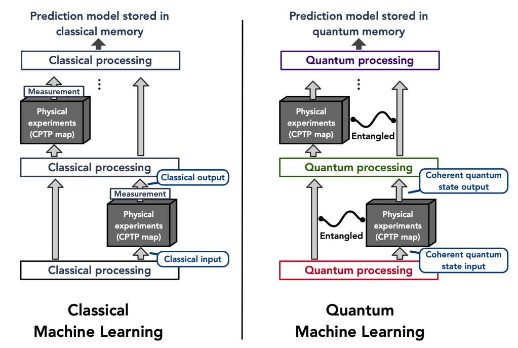


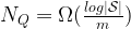


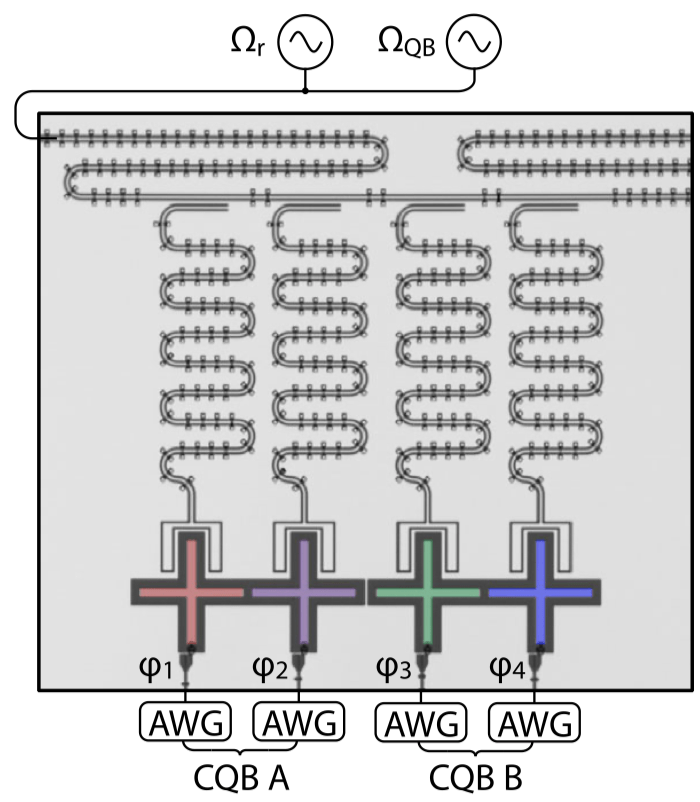
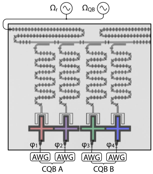
 (
( ) is the reduced magnetic flux that determines the frequency of each transmon, controlled in real time by the arbitrary waveform generators (AWGs);
  and
and  are the microwave control fields for qubit state readout and initialization, respectively.
 and
and  where
where  denotes the transmon index. A single transmon qubit has frequency
  –that is, the energy difference between its ground state
  and the excited state
  . This frequency
  threading the
  where
where  is the magnetic flux quantum. As two transmons are flux-tuned to
  and
and  they should have the same frequency
  . But instead of their energy levels crossing an energy gap called an “avoided crossing”appears for the coupled transmons (solid lines in the plot below). The magnitude of the avoided crossing
  is 65 MHz in this device, and it depends on the coupling strength between two transmons. (For an intuitive and pictorial explanation of avoided crossings, I recommend
 65 MHz appears at
  when two transmons are biased at the same frequency
  .
. . By this definition, the composite qubit has the frequency of the gap
  , with states
  and
and  associated with the eigenstates of
  , and the bare transmon states
  and
and  associated with the eigenstates of
  . The parameter
  in the second term is determined by the frequency difference between the two bare transmons
  , and is controlled by varying the flux biases on the individual transmons simultaneously as a function of time. As we expect, at the composite qubit operating point
  , the qubit exhibits an energy splitting of
  , let’s denote its instantaneous eigenstates as
  and
and  , corresponding to the lower and the higher energy eigenstates, respectively. The
  from state
  and depends on the size of the avoided crossing
  . (For a pedagogical derivation of this formula, see
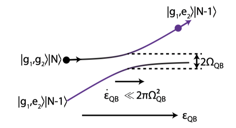
 and amplitude
  (corresponds to the filled in black circle in the figure above). This is achieved by waiting a sufficient time for the transmons reach the thermal equilibrium as the transmon temperature (around 40 mK at the bottom of the dilution fridge) is much smaller than their energy gaps (around 7 GHz for both transmons) so that
  and the transmon thermal state is approximately its ground state. Then turn on a static coherent microwave drive field of frequency
  ; this drive hybridizes the states
  and
and  as shown in the diagram above, and causes a splitting with magnitude
  in the qubit energy spectrum. This splitting is known as
  of transmon 2 by tuning its flux bias
  . Let
. Let  be the detuning between transmon 2 frequency and the drive frequency
  , and sweep
 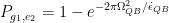 . Thus we see that high-fidelity state initialization requires that the change in transmon 2 frequency be slow enough such that
 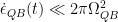 .
. so that the qubit state adiabatically evolves to
  .
. . It takes about 250 ns to complete the above state initialization steps; this is mostly limited by how slow the change of the system needs to be to meet the adiabatic condition
  -,
-,  – and
– and  -axes, respectively. In composite qubits, the single-qubit gates are implemented through the transmon flux controls
  in the transmon circuits. This in turn leads to the time-dependent magnetic fluxes to control the transmon frequency difference
  -gates
 .
. -gate implements a rotation around
  :
:  . The Z-gate of the composite qubit is realized by simply idling the qubit (that is, biasing the qubit with a constant magnetic flux) at the avoided crossing
  for some gate time
  . Governed by the Schrodinger equation, the evolution of the state from the initial state
  to the final state
  after applying Z-gate is given by an unitary operator
  , i.e.,
  , where
 ![U(t_d)=\exp[-iH_z(t_d)]](https://s0.wp.com/latex.php?latex=U%28t_d%29%3D%5Cexp%5B-iH_z%28t_d%29%5D&bg=ffffff&fg=010101&s=0&c=20201002) – this is exactly the unitary we need to realize a
– this is exactly the unitary we need to realize a  .
. and
and  gates
gates as an example; in the Bloch sphere representation, this gate rotates the qubit state about the
  . The schematic below shows the control
  with idling operations (i.e., constant flux biases at the avoided crossing, equivalent to Z-gates) padded before and afterwards.
 denotes how much the flux controls
  (i.e.,
 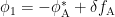 and
and  ), let
  be the instantaneous eigenstates of the time-dependent Hamiltonian
  , and let
 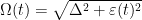 be the energy gap between two states. The plot below shows how the qubit energy gap
  changes with respect to the flux detuning
 :
: (
( (
( ) phase accumulates between the two qubit eigenstates.
 (
( (
( ) phase accumulates between the qubit eigenstates (the same as what happened during
  (
(
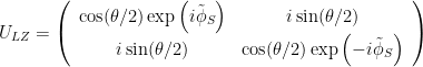 . Thus, the occupation amplitude in the upper and lower eigenstates interfere, resulting in the state transitions with the probability
  , and a relative phase
  introduced between
  . Geometrically this can be interpreted as the area under the curve
  (the shaded blue area above).
 pulse, once chosen, establishes an x-axis of the Bloch sphere. The
  gate, a rotation around y-axis, is then implemented by advancing the onset of the
  which corresponds the gate time of a
  gate, i.e.,
  , as shown below.
 = 125 MHz (corresponds to a 8 ns sine pulse). The frequency of the sine pulse (thus determines the gate time) is chosen such that the passage through the avoided crossing is fast enough to induce LZ transitions, but also not too fast so fast that successive LZ transitions overlap with each other. The flux control can be easily realized using an arbitrary waveform generator. Compared with the Rabi-type of gates where one needs to modulate the microwave signal at several gigahertz which require expensive microwave generators and IQ mixers, the type of gates here using LZ interference are simpler and cheaper to implement in the hardware.
  interaction between two composite qubits. This interaction is realized by adiabatically tuning the frequency of the second composite qubit to realize an avoided crossing that evolves the second excited state of the bare transmons – this operation is similar to how a CZ gate is implemented between two standard transmon qubits. The composite qubit state is read out by uniquely mapping the computational states
  and
and  by the adiabatic evolution, and then read out through the readout resonators as in standard transom qubits.
 and the latter
  ) are sources of errors in a single transmon qubit. However, to cause a transition between the qubit computational states
  time measures the timescale on which state transition between qubit states occurs. The measured
  , which measures the time scale on which the qubit goes from a maximal superposition state to a classical probability mixture. The
  s which is much larger than the
  qubit
qubit
 then the phase relationship between the two terms will remained well defined, i.e. there is no “dephasing” noise. The time for an equal superposition state,
  , to completely dephase to an orthogonal state,
  , is known as “T2 coherence time” or “dephasing time.”
 . If there are
  ions in this trap, then, just like coupled harmonic oscillators, the system is defined by the
  normal modes of motion shared among the ions in the trap. This means that, because the ions are electrically charged and thus through their Coulombic repulsion the motion of one ion affects the motion of another, we can use this interaction to couple qubits together—as an information bus for multi-qubit gates.
 , then we can drive this sideband transition by applying a laser whose frequency
  , where
  is qubit frequency splitting and
  is one of the shared motion normal mode frequencies. Depending on whether we choose a positive or negative detuning, this will cause a blue sideband transition up to
  or a red sideband transition to
  , respectively. In this way we can add and subtract single phonons from the trapped ion system, which can allow us to cool the system to the ground state of motion and also move information from the electronic state of one ion to the electronic state of another by transferring it through their shared motional mode.
  , then applying a red sideband will do nothing, since there is no motional energy level lower than
  , which is necessary to satisfy energy conservation in this case. The same reasoning can be applied for the case where we try to apply a blue sideband pulse on a starting state
  —there is no motional state below
  , so the blue sideband does nothing to this state. See the figure below for a pictorial representation:
 ,
,  , and
, and  (where
  are the qubit levels and
  is an auxiliary level) Cirac and Zoller proposed the following three steps:
  and
and  on ion 1. This will move the population in state
  to state
  -pulse between
 and
and  on ion 2. If a quantum of motion was added in step 1, then this will cause a transition between
  and
and  . Since it is a
  back to
  , leaving the system back in the ground state of motion.
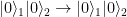


 , and the “cost” is the energy of the state. The function is characterized by a linear operator
  (usually a Hamiltonian). Every
  for every temperature.
  represents the inverse of temperature, so
  is “burning hot,” though for such a tiny device “hot” just means randomly scrambled (i.e. noisy). Likewise,
  is absolute zero temperature, meaning everything is perfectly in order and functioning as intended (i.e. noiseless).
 qubits initialized at state
  attempts to follow the absolute zero temperature path (orange arrow) through the space of “noiseless” quantum states (black Bloch sphere) and arrive at the true answer
  . However, the real computation takes a noisy path (black arrow) that after enough time, leads to the steady state of the noise at
  .
.  is too difficult to simulate classically (NP complexity), but at each intermediate state
  . One of those equal-energy states is the Gibbs state at temperature
  . In fact, we can “mirror” the real path of the quantum device (black arrow) as it progresses in time by matching all intermediate states with Gibbs states, producing a “mirror descent” (green line) from the correct answer to the steady state of the noise
  .
.  below which we are guaranteed to efficiently classically compute the Gibbs state, providing a cost function estimate better than the current quantum state
  . Once a quantum computation passes the threshold( i.e. has an equivalent Gibbs state at with
  ), one has certified classical superiority. All that remains to use this technique is a method for quantifying how far along in
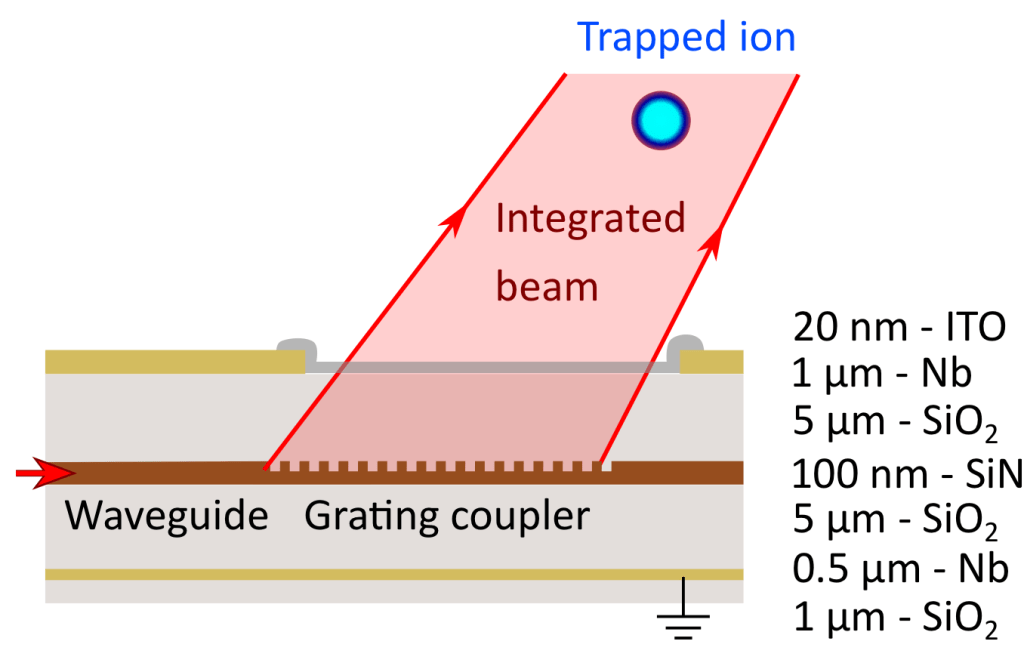
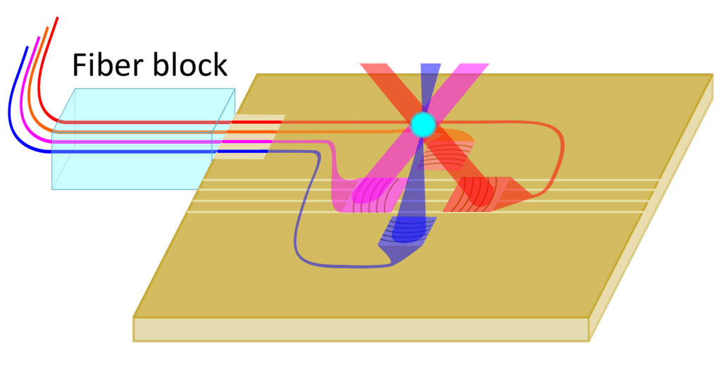


 applications of a classical primitive circuit (also called an ‘oracle’), and a quantum algorithm solving the same problem making only
  calls to a quantum oracle.
 polynomial quantum speedup. If a call to the quantum oracle takes time
  and the classical oracle call takes time
  , then realizing a quantum speedup requires that
 .
. is the fraction of the algorithm’s runtime that cannot be parallelized and
  is the number of processors used, then the runtime can be reduced by a factor
 .
.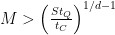
 ,
,  and 2) a specific algorithm for solving the
 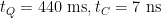 . The ‘lower bound’ gives an estimate for the best speedup that can reasonably be achieved using Google’s quantum computing hardware, while the simulated annealing example is meant to ground their estimates with a specific, practical algorithm which has already been studied in depth. This results in the following table (Table 1 in the paper), where
  is the total runtime required to realize a quantum speedup, given for several values of
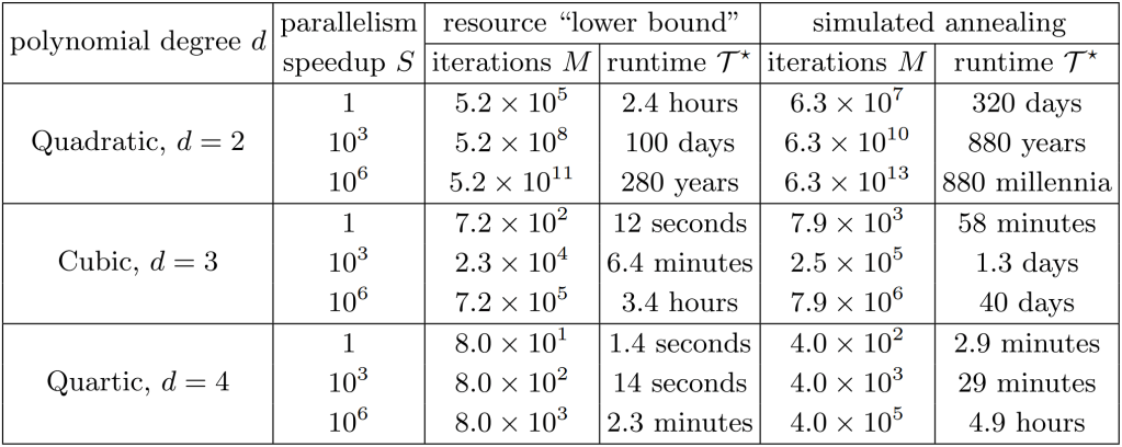

 over the continuous parameter
  , the standard deviation
  is defined as the square root of the variance
  . Here
  and
and  are the first and second moments of the distribution
  . Note here that the 0th moment is just the requirement for normalization
  , and that the limits of integration run over the full range of the parameter
  , it is straightforward to define moments of a discretized distribution
  where
where  is now a discrete probability distribution (and must be normalized accordingly).
 away from the mean value
  (which is also the first moment, see the preceding paragraph), the height of the distribution is reduced by a factor
  from its maximum, where
  is Euler’s number. If one has the explicit form of the Gaussian distribution
 , for reasons that will be clear momentarily) than the other. As such, the distribution with the larger half-width (dashed) yields a lower probability to observe the parameter
 . Here,
  is the operator describing the excited state population of the two-level system (generically, this can be bosonic if we limit ourselves to the single-excitation Hilbert space),
  is the
  is the resonance frequency of the two-level system. All this is to say the following: if we start the system in the excited state at some time
  and let it decay, the light emitted by the two-level system will have a Lorentzian profile! So this is a distribution of physical meaning and interest, and we’d like to have a measure of uncertainty that can describe it!
 , where
  is the probability to observe the (discrete) value
  . Now we run into an issue: both the variance and the average value depend on the ordering of the values
 and
and  . They each occur with probability
  , so that the average value is
  and the standard deviation is
  . But if we relabel our distribution so that our two outcomes are now
  and
and  , the standard deviation changes to
  . In both cases, there are two outcomes with the same probabilities, and we are learning the same amount of information. Why is our uncertainty changing? Well, the standard deviation is an average measure of the distance of each point from the average value–an average value that may not even be in the original distribution, let alone be its maximum as it is for the Gaussian distribution!
 . Although the choice of logarithm is arbitrary, I prefer base
  so that the entropy is the average amount of information conveyed by an outcome measured in bits. In the case of the two equal-outcome distribution, the entropy is
  ; one bit of information remains concealed. Similarly, if an outcome is known to occur with unit probability the entropy of the distribution is
  ; no information is revealed, since we already knew what the outcome would be! In the event that there are more than two equally outcomes, the entropy increases accordingly (corresponding to a broader distribution). And since the sum of probabilities times their logarithms has no dependence on the parameter labels, the entropy does not suffer from the label permutation problem.
  , we can define the uncertainty of a continuous parameter
  by
by  , where
  is the bin size for our continuous parameter and
  is the Shannon entropy associated with the measurement outcome
  . Here
  is precisely the sort of probability distribution discussed in the prior discrete case example. The posteriori probability distribution
  th bin of size
  measures the number of bins that the measurement underdetermines, and then scales that number of bins by the width of each bin to generate a resolution with the appropriate units!
  , this uncertainty definition is bin size independent! Additionally, it leaves the familiar Heisenberg limits of quantum mechanics take on a very nice form; for instance, if we consider a simultaneous measurement on the position
  of a quantum particle, the sum of the two associated Shannon entropies is bounded for each measurement outcome
 ![[H_x^{(k)} + H_p^{(k)}] > {\rm log}_2(e) - 1 - {\rm log}_2 (\frac{\delta x \delta p}{h})](https://s0.wp.com/latex.php?latex=%5BH_x%5E%7B%28k%29%7D+%2B+H_p%5E%7B%28k%29%7D%5D+%3E+%7B%5Crm+log%7D_2%28e%29+-+1++-+%7B%5Crm+log%7D_2+%28%5Cfrac%7B%5Cdelta+x+%5Cdelta+p%7D%7Bh%7D%29&bg=ffffff&fg=010101&s=2&c=20201002) with
with  Planck’s constant and
  and
and  the bin-sizes for position and momentum, respectively . Clearly this bound on the Shannon entropies is not bin-size independent. However, directly inserting this bound into the expression for the uncertainties themselves, we find that
  . (For a thorough derivation, see
  (calculated using
  bins of size
  ). Now the uncertainty is directly proportional to the half-width half-max of the distribution
  . Regardless of the separation between the bins, the distribution is over the same amount of parameter space. Distributions that move further apart in this way are of physical relevance; indeed, the simple distribution above could be considered a very crude model of Rabi splitting. Two Lorentzians moving apart would be a more accurate model, and would also display the separation-independence we are interested in here.
  nd law of thermodynamics, which states that entropy always increases within a closed system at thermal equilibrium. This is because learning necessarily occurs in a system that is not closed! Of course a classical memory register’s entropy will never decrease in the absence of inputs, because inputting the outcomes of measurements is how learning occurs!
  ), whereas the fastest classical algorithms all scale polynomially (
 ). There is a subtlety involved, though, since the solution to the ODE is encoded in the amplitudes of a quantum state
 qubits. We want to solve a differential equation of the form:
 is a
is a  matrix and polynomial function of
  given the initial state as input.
  . The corresponding quantum state is
 ,
, is the i’th computational basis state. As usual, the quantum state requires only log(d) qubits to represent the d basis vectors. Notice, however, that if we wanted to obtain a classical representation of x from
  , we would need to conduct O(d) measurements of the quantum state. This is a major caveat to the non-linear ODE algorithm; although the algorithm itself runs in polylog(d) time, extracting the full solution takes poly(d) time. Nevertheless, you can extract some useful information like power spectra from such a state efficiently, maintaining the exponential advantage.
 and
and  is anti-Hermitian, that is,
 is the solution to the ODE at timestep
  .
. in the output for total simulated time T and a timestep of
  ,
, is the average norm squared of the eigenvalues of the ‘non-Hermitian Hamiltonian’ f over the total simulation time – this is reasonable provided either that the eigenvalues don’t grow exponentially fast or we solve for sufficiently short times; essentially this means the algorithm works well for systems that aren’t chaotic. Again, this doesn’t necessarily mean that quantum computers will replace classical computers for solving non-linear ODEs in all cases, but it may well open the door to some exciting applications down the line!