Uncertainties Regarding Uncertainties: Modern Lessons from Entropy and Quantum Information Theory

These are uncertain times, so let’s talk about uncertainty. In particular, I would like to focus on how we quantify uncertainty, focusing on the failings of our most common quantifier of uncertainty (the standard deviation) and singing the praises of alternative entropic measures of uncertainty. This not only impacts how we think about uncertainty, but also how we understand the information-theoretic process of learning itself. I’ll come back to this at the end.

So, what is uncertainty, and how do we quantify it?

One of the most common ways to define and quantify uncertainty is through the standard deviation or root mean squared error. For an arbitrary classical probability distribution $f(x)$ over the continuous parameter $x$ , the standard deviation $\sigma$ is defined as the square root of the variance $\sqrt{\left<x^2\right> - \left<x\right>^2}$ . Here $\left<x\right>$ and $\left<x^2\right>$ are the first and second moments of the distribution $f(x)$ , respectively. Although there’s no need for higher moments in calculating the standard deviation, we may as well define all the moments of $f(x)$ in one fell swoop: $\left<x^n\right> = \int dx f(x) x^n$ . Note here that the 0th moment is just the requirement for normalization $1 = \int dx f(x)$ , and that the limits of integration run over the full range of the parameter $x$ . Similarly, if $x$ is replaced with a discrete parameter $x_i$ , it is straightforward to define moments of a discretized distribution $\left<x_i^n\right> =\sum\limits_i f(x_i) x_i^n$ where $f(x_i)$ is now a discrete probability distribution (and must be normalized accordingly).

Does this definition of uncertainty seem clunky and non-amenable to calculation? Fear not, enter our humble friend, the Gaussian distribution.

The Gaussian distribution (also known as the normal distribution, especially in the social sciences) is perfectly amenable to the standard deviation as a measure of its uncertainty. First and foremost, the standard deviation has a clear physical interpretation; at one standard deviation $\sigma$ away from the mean value $\mu$ (which is also the first moment, see the preceding paragraph), the height of the distribution is reduced by a factor $\frac{1}{\sqrt{e}}$ from its maximum, where $e$ is Euler’s number. If one has the explicit form of the Gaussian distribution $f(x)$ , one doesn’t even need to use the formulas above, one can just read off the standard deviation! Conversely, a Gaussian distribution is completely characterized by its mean value $\mu$ and its standard deviation $\sigma$ . So if one is sampling from a Gaussian distribution, it is straightforward to estimate the distribution itself from the statistical properties of the measurements.

Now by incredible coincidence, the Gaussian distribution appears in two vastly different contexts in Physics: as the average of many independent random variables as per the central limit theorem, and as the minimum uncertainty state in quantum theory. (It’s actually no coincidence at all, but that must be saved for a different article.) These are two very important contexts, but this is not exhaustive. There are many other contexts in Physics, and there are other distributions besides the Gaussian. And critically, the standard deviation is not a universally good measure of uncertainty. To clarify this, let’s look at an example.

In the above plot we have two normalized Lorentzian or Cauchy distributions, one with a larger half-width (denoted for the Lorentzian by $\gamma$ , for reasons that will be clear momentarily) than the other. As such, the distribution with the larger half-width (dashed) yields a lower probability to observe the parameter $x$ at the location parameter $\mu$ , and a higher probability to observe the parameter $x$ over a broader range of values. So any reasonable universal measure of uncertainty should assign a higher uncertainty to the broader distribution than to the narrower one. Does the standard deviation do this? No it does not! It assigns them the same uncertainty, which is infinity! The long tails of the Lorentzian result in a variance which is infinite, and the square root of infinity is still infinity!

Of course, at this point you may object that the Lorentzian distribution is a pathological example and that this argument is a strawman, and you would be right. After all, the Lorentzian doesn’t even have a well-defined average value, why would we expect it to have a sensible variance? Nonetheless, the Lorentzian is not an obscure and oft-forgotten distribution, especially in quantum optics. On the contrary, it plays a key role in describing the physicist’s second favorite model after the simple harmonic oscillator: the two-level atom.

A two-level system coupled to a flat (Markovian) electromagnetic continuum of states

The Lorentzian appears naturally as the homogenous solution to the Quantum Langevin equation $\partial_t \hat{a}(t) = - i\omega_0 \hat{a}(t) - \frac{\gamma}{2} \hat{a}(t) - \sqrt{\gamma} \hat{a}_{\rm in}(t)$ . Here, $\hat{a}(t)$ is the operator describing the excited state population of the two-level system (generically, this can be bosonic if we limit ourselves to the single-excitation Hilbert space), $\hat{a}_{\rm in}(t)$ is the input operator describing excitations in the flat (Markovian) continuum external to the two-level system, $\gamma$ is the incoherent coupling between the two-level system and the continuum of states, and $\omega_0$ is the resonance frequency of the two-level system. All this is to say the following: if we start the system in the excited state at some time $T$ and let it decay, the light emitted by the two-level system will have a Lorentzian profile! So this is a distribution of physical meaning and interest, and we’d like to have a measure of uncertainty that can describe it!

Let’s consider another example–one that will bring us closer to our goal of finding a better measure of uncertainty.

Consider a discretized distribution $\{p_{x_i}\}$ , where $p_{x_i}$ is the probability to observe the (discrete) value $x_i$ normalized such that $\sum_i p_{x_i}=1$ . Now we run into an issue: both the variance and the average value depend on the ordering of the values $x_i$ . To see what I mean, consider again our friend the Gaussian and let’s imagine rearranging it slightly (achievable easily in photoshop).

Here we have swapped the two shaded regions of the Gaussian, changing both the mean and also the average distance from the mean, that is, the standard deviation. But notice, the area underneath the curve remains unchanged! If we imagine discretizing this distribution and sampling from it randomly, the probability distribution $\{p_{x_i}\}$ remains unchanged, except for the reordering of some of the outcomes $x_i$ ! In other words, we learn the same amount of information about both the swapped and unswapped distributions with each sampling. And this issue persists in the limit of a continuous distribution too!

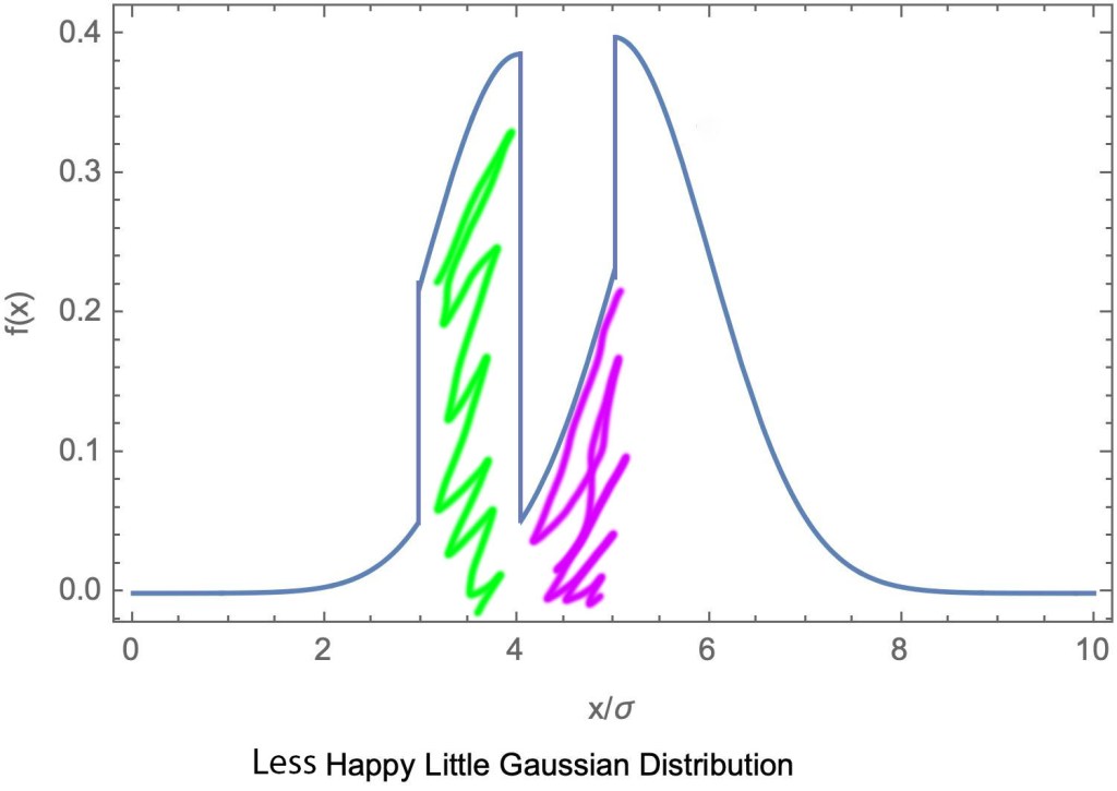
To really drive it home, let us consider a very simple example: a distribution consisting of two outcomes for a variable $x=1$ and $x=2$ . They each occur with probability $1/2$ , so that the average value is $x_{\rm avg}=1.5$ and the standard deviation is $\sigma = .5$ . But if we relabel our distribution so that our two outcomes are now $x=0$ and $x=3$ , the standard deviation changes to $\sigma = 1.5$ . In both cases, there are two outcomes with the same probabilities, and we are learning the same amount of information. Why is our uncertainty changing? Well, the standard deviation is an average measure of the distance of each point from the average value–an average value that may not even be in the original distribution, let alone be its maximum as it is for the Gaussian distribution!

So what do we do? What can we use if not the standard deviation? Is there some other measure of uncertainty with a clear physical meaning that doesn’t suffer from this issue when outcomes are permuted? One that will always gives us a sensible answer for both discrete and continuous probability distributions?

The Solution: Entropic measures of Uncertainty

Enter Claude Shannon, father of information theory.

Claude Shannon - Wikipedia — Dr. Claude Shannon, image courtesy of wikipedia

Given a normalized distribution $\{p_{x_i}\}$ , with $p_{x_i}$ is the probability to observe $x_i$ , the Shannon entropy is defined $H_x = -\sum\limits_i p_{x_i} {\rm log} p_{x_i}$ . Although the choice of logarithm is arbitrary, I prefer base $2$ so that the entropy is the average amount of information conveyed by an outcome measured in bits. In the case of the two equal-outcome distribution, the entropy is $1$ ; one bit of information remains concealed. Similarly, if an outcome is known to occur with unit probability the entropy of the distribution is $0$ ; no information is revealed, since we already knew what the outcome would be! In the event that there are more than two equally outcomes, the entropy increases accordingly (corresponding to a broader distribution). And since the sum of probabilities times their logarithms has no dependence on the parameter labels, the entropy does not suffer from the label permutation problem.

There are many reasons to love the Shannon entropy as a stand-alone quantifier of uncertainty. Unlike the standard deviation which always has the units of the variable it describes, the entropy is unitless. This allows for natural comparisons between different parameters free of reparameterization. And the entropy has a natural interpretation: the number of yes/no questions needed (on average) to determine the value of a parameter (to the resolution determined by the bin size, as we will come back to very shortly). While the interpretation of the entropy as a measure of bits changes if a different base is used for the logarithm, the approach is still the same. And for a parameter that is truly discrete, the Shannon entropy is simply the best measure of uncertainty. In my work in photo detection theory, such a parameter of interest is the number resolution in a photo detector. (Here there is a slight complication; the probability that appears is the conditional posterior probability, which can be calculated through Bayes theorem.)

However, we are not only interested in discrete quantities but also continuous ones. And in these cases, what we want from an uncertainty measure is a quantifier of the resolution provided by an outcome–that is, providing a range of likely values for an arbitrary (read: non-Gaussian) distribution. Here is the procedure for generating such a measure, following closely Białynicki-Birula‘s method, building upon the pioneering work by Helstrom, Białynicki-Birula, and Mycielski.

For a measurement outcome $k$ , we can define the uncertainty of a continuous parameter $X$ by $\Delta X^{(k)} = 2^{H^{(k)}_X} \delta X$ , where $\delta X$ is the bin size for our continuous parameter and $H^{(k)}_X$ is the Shannon entropy associated with the measurement outcome $k$ . We can define this Shannon entropy in terms of a posteriori probability such that $H_X^{(k)} =-\sum\limits_j p(j|k) {\rm log}_2 p(j|k)$ . Here $p(j|k)$ is precisely the sort of probability distribution discussed in the prior discrete case example. The posteriori probability distribution $p(j|k)$ is the probability that, given a measurement outcome $k$ , the input had parameter $X$ in the $j\!$ th bin of size $\delta X$ . In this way, the measurement uncertainty $\Delta X^{(k)}$ measures the number of bins that the measurement underdetermines, and then scales that number of bins by the width of each bin to generate a resolution with the appropriate units!

It is simple to see that this definition of uncertainty is independent of the ordering of the bins, but perhaps more surprising is that, in the limit that the bin sizes approach zero $\delta X\rightarrow 0$ , this uncertainty definition is bin size independent! Additionally, it leaves the familiar Heisenberg limits of quantum mechanics take on a very nice form; for instance, if we consider a simultaneous measurement on the position $x$ and momentum $p$ of a quantum particle, the sum of the two associated Shannon entropies is bounded for each measurement outcome $[H_x^{(k)} + H_p^{(k)}] > {\rm log}_2(e) - 1 - {\rm log}_2 (\frac{\delta x \delta p}{h})$ with $h$ Planck’s constant and $\delta x$ and $\delta p$ the bin-sizes for position and momentum, respectively . Clearly this bound on the Shannon entropies is not bin-size independent. However, directly inserting this bound into the expression for the uncertainties themselves, we find that $\Delta x \Delta p \geq \hbar e \pi$ . (For a thorough derivation, see Białynicki-Birula, building off earlier work by Maassen and Uffink.)

Let’s apply our new uncertainty measures to two of the examples we’ve discussed here. First, let’s revisit our pathological friend the Lorentzian distribution. Now, it is straightforward to calculate the entropic uncertainty, which we find to be $\Delta x \approx 4.9 \gamma$ (calculated using $200$ bins of size $\delta x = 0.1 \gamma$ ). Now the uncertainty is directly proportional to the half-width half-max of the distribution $\gamma$ , as we would intuitively expect it to be.

Let’s also reconsider the two equal-outcome distribution. If we consider these two outcomes to describe two non-overlapping bins of a continuous parameter $x$ each with bin-width $\delta x$ , then the uncertainty is simply $\Delta x = 2\delta x$ . Regardless of the separation between the bins, the distribution is over the same amount of parameter space. Distributions that move further apart in this way are of physical relevance; indeed, the simple distribution above could be considered a very crude model of Rabi splitting. Two Lorentzians moving apart would be a more accurate model, and would also display the separation-independence we are interested in here.

(Here I would like to note that two Gaussians moving away from each other would also have a separation independent entropic uncertainty. Moreover, their variance would be separation independent as well! This is not true for the other distributions discussed above, and is a unique feature of the Gaussian; the reason has to do with the differences between local and global smoothness under scaling transformations, as is outside the scope of this review. All this is to say, the standard deviation really is a good measure of uncertainty for the Gaussian, and credit should be given where it is due!)

This concludes most of what needs to be said here about entropic uncertainty measures; for discrete parameters, the Shannon entropy naturally characterize missing information, and for continuous parameters it is straightforward to generate a resolution measure directly from the Shannon entropy. If you are new to entropic uncertainty measures, hopefully you now feel a little more prepared to understand their usage and necessity. If you’d like to learn more about entropic uncertainty relations and their uses, I highly recommend this wonderful review article. In particular, entropic uncertainties come into play in quantum cryptography (the study of cryptography protocols making use of quantum correlations i.e. quantum key distribution) , quantum metrology, and measurement theory more broadly. Here, there is a natural connection between the entropy and the Fisher information; the Fisher information is a measure of how much of the variance is removed after collecting a single point of data, so that a high-entropy measurement has a low Fisher information.

As a final offering of further reading, if you’re interested in understanding how entropic uncertainty measures can connect the information-theoretic description of a photo detection experiment to industry-standard photo detector figures of merit, this paper (which laid the groundwork for my current understanding, along with my PhD dissertation) should now be fully understandable to you.

I want to end on a more philosophical note discussing entropy, thermodynamics, quantum measurement, and the physical nature of learning.

In quantum theory, a measurement defined by Kraus operators and a POVM is what connects a quantum state to a classical memory register. In other words, it’s how we learn about the quantum world. The quantum states we are trying to learn about are themselves distributions over parameters, and so a Bayesian approach to learning about these distributions is natural (compared to a frequentist’s approach, for instance). In doing quantum measurements, we are trying to update our classical information encoded in bits to accurately describe the quantum distributions in the external world. In the absence of prior knowledge about a quantum state, we start with a high-entropy distribution and move towards a lower and lower entropy distribution as we sample the quantum state. Entropy is the connection between these two distributions, and we can understand its role in our theory as interpolation; the uncertainty of our (classical) distribution is constrained by the entropies associated with the state we are trying to measure and the quantum measurements we perform on that state. (We should also note that inclusion of a classical memory is not necessary for a definition of entropy and a quantum memory can be used as well, as discussed in the aforementioned review article.) We lower the entropy of our distribution by learning. This does not violate the $2\!$ nd law of thermodynamics, which states that entropy always increases within a closed system at thermal equilibrium. This is because learning necessarily occurs in a system that is not closed! Of course a classical memory register’s entropy will never decrease in the absence of inputs, because inputting the outcomes of measurements is how learning occurs!

Learning requires openness to new information; this holds true as both a statement about human nature and about quantum systems. Open quantum systems are not just a handy way to incorporate the inconvenient effects of decoherence. They are a general framework for understanding information flow in quantum theory, and an essential ingredient to any quantum theory in which learning can occur.

I would like to thank MaryLena Bleile at Southern Methodist University as well as Anupam Mitra at the University of New Mexico’s Center for Quantum Information and Control (CQuIC) for their helpful conversations about entropy and quantum uncertainty. I would also like to offer deep gratitude to Dr. Steven van Enk at the University of Oregon who, during our work together on photo detection theory, introduced me to entropic uncertainty measures and showed me their light.

Dr. Tzula Propp is a postdoctoral researcher at the University of New Mexico’s Center for Quantum Information and Control (CQuIC). Their work in quantum optics and quantum information theory focuses on quantum measurement, quantum amplification, and non-Markovian open quantum systems.

The Solution: Entropic measures of Uncertainty

Share this:

Like this:

Leave a Reply Cancel reply