Quantum systems are generally very sensitive, and upon interacting with the environment, their quantum properties can decohere. This essentially makes a given quantum system dissipate into purely classical behavior. However, in certain contexts it is possible to use dissipation in a controlled fashion to increase the control of quantum systems. A few examples of controlled dissipation in this way include laser cooling of atoms, cooling of low frequency mechanical oscillators, and for the control of quantum circuits. In this recent publication [1], the authors are able to demonstrate stabilization of superposition states in a superconducting qubit using a custom made photonic crystal loss channel. By considering how the photonic crystal induces loss on the system, the authors provide a master equation treatment which explains how the combination of a specialized drive applied to the qubit in addition to the dissipation provided via the photonic crystal allows for precise control of the qubit state for times much longer than standard qubit coherence times.
Experimental Details
This experiment consists of a superconducting qubit whose dipole moment is coupled to the electric field inside of a three dimensional waveguide cavity. In this experiment, the role of the waveguide cavity is to provide microwave control of the qubit as well as reading out the state of the qubit. The superconducting qubit consists of two Josephson junctions in parallel, forming a superconducting quantum interference device (often referred to as a “SQUID”). This allows the authors to change the resonant frequency of the qubit by threading an external magnetic field through the SQUID loop. On the output of the waveguide cavity, the authors connect a photonic crystal to the circuit. This photonic crystal is made out of a regular coaxial cable which is mechanically deformed in a specific way in order to change the impedance of the cable. The result of the spatially varying impedance in the cable leads to the opening of a bandgap – leading to photon energies (or frequencies) where the photonic density of states is zero (see Fig. 1 for a schematic of the experimental setup). By changing the photonic density of states as a fucntion of energy, the decay of the qubit will also change as a function of frequency.
Figure 1 Left: Schematic of the experimental system. The superconducting qubit is mounted in a copper cavity which is used for control and readout of the qubit state. By passing current though a superconducting wire wrapped around the cavity a magnetic field is generated perpendicular to the substrate containing the qubit, allowing the authors to tune the resonant frequency of the qubit. The photonic crystal is connected to the output port of the cavity, changing the density of states that the qubit can decay into. Right: Room temperature measurements of the reflection off of the photonic crystal. In the stop-band (from 5.5 – 6.4 GHz) most of the signal sent into the photonic crystal is reflected, verifying that there is a low density of states at those frequencies. Above 6.4 GHz, the photonic band gap closes and photons can transmit through the photonic crystal.
Qubit Decay Rates
In order to measure the decay rate of the qubit, the authors first excite the qubit into its excited state by applying a pulse of energy which is resonant with the qubit to the system. They then measure the probability of the qubit remaining in its excited state as a function of time after the pulse is applied. By fitting the measured probability to an exponential decay and extracting the decay constant, one is able to determine the qubit decay rate. The resonant frequency of the qubit is then adjusted by changing the external magnetic flux threading the SQUID loop, and measuring the qubit decay rate as a function of qubit frequency in order to investigate the impact of the photonic crystal on the qubit lifetime. The total decay rate of the qubit can be written as
In Eq. 1, is the measured decay rate of the qubit, is the linewidth of the microwave cavity, is the coupling strength between the qubit and the cavity, is the difference in resonant frequency between the qubit and the cavity, is the density of states of the photonic crystal at the qubit frequency, and represents decay of the qubit into dissipation channels other than the photonic crystal. By measuring the total qubit decay rate for various values of , it should be possible to extract information about the density of states of the photonic crystal! See Fig. 2 below for the resulting measurement
Figure 2 Measurement of qubit decay rates over a broad range in frequencies. Because the qubit loss varies quickly with qubit frequency, by flux biasing the qubit to a point where the derivative of the qubit loss is large, it is possible for Mollow triplet sidebands to sample frequencies with both very high and very low loss. By measuring the generalized Rabi frequencies across the same values of qubit frequency, the authors verify the variable couple of the qubit to the photonic crystal.
Dynamics and Emission of a Driven Qubit
After verifying that the density of states in the photonic crystal can shape the decay rate of the qubit, the authors now consider more carefully how the qubit actually emits energy. Specifically, a strong drive applied with amplitude which is detuned from the qubit energy by , where is the frequency of the drive and is the qubit energy is considered. If the amplitude of the drive is much larger than the loss rate of the qubit, the qubit will emit energy at three different frequencies , and , where is called the generalized Rabi frequency. This emission spectrum is called the Mollow triplet [2]. See Fig. 3 for a schematic of the Mollow triplet emission.
Figure 3 Schematic which represents the emssion of the driven two level system. Under the presence of a strong drive, the qubit emits radiation at frequencies corresponding to the drive frequency as well as at the frequencies . Due to the shaped loss spectrum, the area of one sideband can be supressed, indicating that the qubit will emit radiation at this frequency at a lower rate compared to the other sideband. Top right: under the presence of the drive, the quantization axis of the qubit also rotates, which changes which qubit states can be prepared/stabilized.
Because the authors have observed that the photonic crystal shapes the loss rate of the qubit on a energy scale comparable to values of experimentally accessible , it is possible for one of the sidebands of the Mollow triplet to experience a high loss rate while the other sideband of the Mollow triplet experiences a low loss rate.
The next thing to consider is what the presence of an applied drive does to the energy spectrum of the qubit. In a frame rotating with the drive frequency, the qubit Hamiltonian is given by
where and are Pauli matrices. Since this Hamiltonian is not diagonal, it is convenient to rotate basis such that the Hamiltonian can be written in a new form
where the rotated Pauli Z matrix can be written as , and the rotation angle is defined as with . Because we have written the Hamiltonian in a rotated basis, we must also consider how the new eigenstates of the system rotate relative to the original eigenstates, which we will call and for ground and excited state, respectively.
At this point it’s probably useful to consider a useful example! In the case of a resonant drive, , which immediately informs us that , so we can rewrite the rotated eigenstates of the system as , and , which have the special property that . Because the state has a lower energy, it will emit energy corresponding to the lower energy sideband of the Mollow triplet and vice versa for the state . If the loss of the qubit is vastly different for either of these states, that will promote decay into either the state or ! Specifically, if the qubit is at a resonant frequency near 6.4766 GHz (see Fig. 2), the state at higher energy (corresponding to in this example) has a lower loss rate, so we should expect that while the drive is turned on, the qubit preferentially would decay into this state! This means that the expectation value would tend towards +1 in this scenario! In the case of a uniform loss spectrum, there would be no preferred decay of the qubit and one would expect that all of the qubit expectation values would decay to zero.
Lindblad Master Equation
In the presence of the combined drive and dissipation experienced by the qubit, the dynamics of the reduced density matrix which describes the qubit can be written according to the Lindblad Master equation [3]:
Here, is the reduced density matrix for the qubit, the dissipation superoperator is also introduced as . The rate represents dephasing of the qubit in the basis rotated by , which couples to the operator and transitions between eigenstates in the rotated basis are driven by the “jump” operators which are related to the rates . Similar to the previous example, if the photonic crystal shapes the qubit loss such that , a corresponding rotating frame eigenstate will be stabilized.
Experimental Results
In order to verify that the authors can use the combination of drive and dissipation to prepare and stabilize qubit states, they implement the following bath engineering protocol. First, the qubit is flux biased to a resonant frequency of 6.4766 GHz (as in our example). Then, a coherent drive is applied to the system for nearly (which is much longer than the qubit coherence times in the absence of drive!). During this time, the qubit should preferentially decay to an eigenstate of the rotated system if the Mollow triplet sidebands have different weights. Once the drive is shut off, the expectation value is measured for various combinations of drive parameters. Results are shown below as well in Fig. 4 as comparisons to numerical solutions to the master equation, the authors not only see that the qubit expectation values don’t decay to 0, but also fantastic agreement between the theory and the experiment! Additionally, we can recall our earlier example, and we see that along the linecut of , the expectation value approaches the value of +1 as we expected!
Figure 4 (a) Measurement of as the parameters of the drive change. For certain drive parameters the value of is negative. As the drive parameters are changed, the system crosses through a region of “zero coherence” where the bath engineering protocol no longer works before stabilizing to positive values. (b) Numeric solutions to the master equation under the same drive parameters as (a). The authors observe excellent agreement between the experiments and the numeric solutions. (c) Comparison of horizontal linecuts from (a,b). The authors observe agreement between the measured values (dots) and simulated values (lines) when considering all expectation values for the qubit state ()
Conclusion
In conclusion, the authors are able to demonstrate the fabrication of a spatially changing impedance coaxial cable which acts as a photonic crystal, and in turn controlling the loss spectrum of a superconducting qubit. The authors are then able to leverage this shaped emission spectrum in the context of the master equation to prepare and stabilize non-trivial states of the qubit for times much longer than the coherence times of the qubit.
References
[1] P. M. Harrington, M. Naghiloo, D. Tan, and K. W. Murch, Bath engineering of a fluorescing artificial atom with a photonic crystal, Phys. Rev. A 99, 052126 (2019)
[2] B. R. Mollow, Power spectrum of light scattered by two-level systems, Phys. Rev. 188, 1969 (1969)
[3] G. Lindblad, On the generators of quantum dynamical semigroups, Communications in Mathematical Physics 48, 119 (1976).
Title: Quantum state preparation, tomography, and entanglement of mechanical oscillators
Authors: E. Alex Wollack, Agnetta Y. Cleland, Rachel G. Gruenke, Zhaoyou Wang, Patricio Arrangoiz-Arriola, and Amir H. Safavi-Naeini
Institution: Department of Applied Physics and Ginzton Laboratory, Stanford University 348 Via Pueblo Mall, Stanford, California 94305, USA
Manuscript: Published in Nature[1], Open Access on arXiv
Introduction The field of quantum information sciences contains a multitude of different technologies, including atoms, spins, and defect centers in diamond. This work focuses on two emerging technologies: superconducting circuits and mechanical oscillators. Each system has its advantages, but it is not obvious that any one is the best platform for building a quantum computer, developing quantum sensors, or facilitating quantum communication. To achieve these goals, it is necessary to develop hybrid quantum systems that can utilize the strengths of various quantum technologies.
In this work, the authors demonstrate the ability to couple superconducting qubits to mechanical motion. This establishes the building blocks for a hybrid quantum system that can take advantage of the the best of both systems. The qubit is customizable and easy to communicate with, making it ideal for state initialization and characterization. The mechanical modes are fabricated with small spatial footprints and have long lifetimes, making it possible to scale to larger systems and hold quantum information for long timescales. I will describe how the authors use the coupling between these two systems to both prepare and measure states of mechanical motion using the qubit. I first describe the carefully engineered device that couples one qubit to two mechanical oscillators. Then I discuss the two modes of operation, where the qubit is used to both prepare states of mechanical motion and measure the quantum state of the mechanical mode. Finally, I show how the authors use the qubit as an intermediary to prepare entangled mechanical states across two oscillators.
Device
Figure 1: Coupling a qubit to mechanics. a. Schematic of the device shows a single qubit coupled to two mechanical oscillators at distinct frequencies. b. Optical image of the qubit with the Josephson junctions shown in the inset. The wire coming in from the left carries current to apply a flux to the junction loop. The rectangular pad on the right of the image is the capacitive pad used to link the qubit to the mechanical oscillators. c. Two mechanical oscillators formed in a periodic structure of LiNiO3. Figure adapted from Ref 1.
The device used in this works consists of two mechanical oscillators and a superconducting qubit. The mechanical oscillators are fabricated in thin film lithium niobate (LiNiO3). These oscillators are formed by embedding a defect in a periodic structure of the material, called a phononic crystal. The defect is a mismatch in the periodicity of the structure and confines mechanical motion, preventing acoustic radiation and enabling long mechanical lifetimes. Like electromagnetic radiation, mechanical motion can be quantized. The individual quanta of mechanical motion are called phonons, and the mechanical oscillator can be characterized as a harmonic oscillator with equal energy level spacing. The qubit is made by fabricating an oscillator with superconducting materials. The key element of this circuit is a Josephson junction, which is made of aluminum oxide sandwiched between layers of superconducting aluminum. The junction acts as a nonlinear inductor that modifies the energy level spacing of the oscillator. The energy levels of the usual oscillator (which is a harmonic oscillator) are equally spaced, meaning the transition energy between any two levels is the same. However, with the nonlinear inductor in the circuit, there are no longer equally spaced energy levels, making it possible to uniquely address the two lowest energy levels of the system, ground () and excited (). The two levels form a quantum bit (qubit). The qubit is designed to be tunable in frequency by placing two Josephson junctions in a parallel with each other. By applying a magnetic field using a wire carrying current, a magnetic flux is threaded through the loop to change the qubit frequency.
The qubit and mechanical oscillators are fabricated on separate chips that are placed apart. To couple the qubit and mechanical oscillators, the authors use the piezoelectricy of the lithium niobate film. The mechanical motion of this material produces an accumulation of electric charges onto aluminum pads located on both chips, which are designed to be the capacitive element of the qubit. The qubit capacitor is charged by the motion of the mechanical oscillators, ensuring that the two systems are linked together.
Initializing a mechanical state The authors design the qubit to interact in two different ways with the mechanical oscillators. In the first mode, the qubit is tuned to be on resonance with a particular mechanical oscillator (). Note that the mechanical frequencies of the two oscillators are different, so the qubit can only be in resonance with one at a time. This allows for the direct exchange of energy between qubit and either oscillator at a rate related to the capacitive coupling between the two, 9.5 MHz, 10.5 MHz. The Hamiltonian that describes the interaction between a qubit and mechanical oscillator on resonance the Jaynes-Cummings interaction:
[Equation 1].
and are the creation, annihilation operators for the mechanical oscillator and qubit respectively. When on resonance, the qubit and mechanical oscillator swap their respective states in time 24-26 depending on the particular oscillator.
Figure 2: Swapping qubit and mechanical state. The qubit (Q) is first initialized in it excited state. Once the qubit is brought into resonance with the mechanical oscillator, the two coherently exchange their states. This means the joint state oscillates between and where represents the state of the mechanics and the qubit. In between a full swap, the qubit and mechanical oscillators are entangled together with the joint state .
This swap can be used as a method of mechanical state preparation. The authors first tune the qubit so that it is off resonant from either mechanical oscillator. Then with the mechanical mode containing no quanta, the qubit is initialized so the joint states are , or state. The joint state , describe the phonon number of a particular mechanical oscillator, …, and whether the qubit is in the ground or excited state, . The qubit frequency is tuned to be on resonance with either mechanical mode for a time corresponding to a full swap. When the swap operation is applied to the joint state , the system remains unchanged since both subsystems are in their ground state and there is no energy to exchange. Under the swap, the state becomes as shown in Figure 1. When the qubit is initialized in a superposition state, the joint state is . The swap operation acts on both parts of this superposition leading to the final state . The mechanical oscillator is now in a superposition state, but the state of the mechanical oscillator is not entangled with the qubit state.
Measuring a mechanical state In the second mode of operation, the qubit is off resonance from either mechanical oscillator, usually called a dispersive interaction. The dispersive interaction rate between qubit and mechanical oscillator, , is now set by the direct capactive coupling, , the detuning between qubit and mechanics, , and other qubit parameters. In the limit that the detuning between qubit and mechanics is larger than the the capacitive interaction rate (), the interaction shown in Equation 1 is approximated by the off resonant Hamilitonian:
[Equation 2].
The combination is the operator version of the number of phonons, , in the mechanical oscillator. is the operator version of the qubit state, either or .
Without the interaction between the qubit and mechanics, the Hamiltonian of the just the qubit would look like , where is the transition frequency of the qubit. When we add in the off resonant interaction, the Hamiltonian can be expressed as . By comparing the combined Hamiltonian with the one of just the qubit, we see that the effect of the interaction is to modify the transition frequency of the qubit (represented by everything before the ). So now, the qubit transition frequency is dependent on the number of phonons in the mechanical oscillator (). For every additional phonon in the mechanical oscillator, the qubit transition frequency shifts by .
This interaction is crucial to being able to characterize the state of the mechanical oscillator. Since the different phonon numbers impart a different frequency shift on the qubit, the mechanical state is imprinted on the frequency of the qubit. To resolve the probabilities of different phonon numbers in the mechanical oscillator, a qubit interferometry measurement is performed. The mechanical oscillator is prepared in a Fock state with 0 or 1 phonons or in a superposition of many phonon 0, 1, 2,… Then the qubit is placed in a superposition state and allowed to precess for a variable time, . During this time, the superposition state accumulates a phase at rate if there is one phonon, for two phonons, and so on. The phase accumulated then reflects the probability () that the mechanical oscillator contained zero, one, two, etc… phonons. The qubit state evolves to , where the phase accumulated is . The authors rotate the qubit back into its measurement basis and monitor the final population of the qubit excited state as a function of the interaction time, , and fit the trajectory to the functional form
[Equation 3]
This form includes the phonon number probabilities, , as well as the number dependent precession rate, . It also includes a number dependent phase offset, , and the phonon decay constant, . This captures the dynamics of the qubit trajectory even when the phonon probabilities are changing due to energy decay. The figure below shows an interferometry trace and the fit used to extract the phonon population in the mechanical oscillator. The trace contains a combination of various frequency oscillations each corresponding to a different phonon number. The weight of a particular frequency in the combination represents the probability of the corresponding phonon number to be present in the mechanical state being measured.
Figure 3: Mechanical state characterization. Qubit interferometry is performed in the presence of phonons in the mechanical oscillator. The resulting qubit state trajectory contains information about the probability distribution of phonon numbers. A typical trace is shown here and is fit with the functional form in Equation 3 to determine the phonon content of the mechanical state. Figure adapted from [1].
Entangling two mechanical oscillators With the ability to control and measure the state of each mechanical oscillator, the next step is to prepare a joint state where the motion of the two oscillators is entangled together. We write the joint state of the qubit and two mechanical oscillators as , where the mechanical oscillators can contain phonons, and the qubit can be in either the ground () or excited () state. First the qubit is prepared in its excited state with . A half swap between the qubit and the first mechanical oscillator entangles the two, . This is accomplished by bringing the qubit into resonance with the mechanical oscillator for only half the time required the perform a full swap as seen in Figure 2. Finally, the qubit state is fully swapped with the second mechanical state resulting in the state . This leaves the qubit in the ground state with the two mechanical state fully entangled together .
Future outlook The authors construct a device that couples mechanical motion to a superconducting qubit. The qubit is used to prepare and measure the modes of individual mechanical modes. The authors present a protocol that prepares two mechanical modes, both coupled to the same qubit, in an entangled state. This work demonstrates the building blocks needed to construct a hybrid quantum system by combining two disparate quantum systems. The authors match the precise control of a superconducting qubit with the long lifetimes of the mechanical modes to construct a devices that engages the strengths of both systems. This kind of design will enable future advances in quantum computing, sensing, and communication by drawing from many different technologies.
References
[1] Wollack, E.A., Cleland, A.Y., Gruenke, R.G. et al. Quantum state preparation and tomography of entangled mechanical resonators. Nature604, 463–467 (2022).
Akash Dixit builds superconducting qubits and couples them to 3D cavities to develop novel quantum architectures and search for dark matter.
Thanks to Joe Kitzman for great discussions and feedback in editing this article.
Superconducting qubits are a promising candidate for functional quantum computation as well as investigating fundamental physics of composite quantum systems where superconducting qubits are coupled to other quantum degrees of freedom. The most common example of this is circuit quantum electrodynamics (cQED), where a superconducting qubit is coupled to an electromagnetic resonator, and the resonator can be used to control and read out the quantum state of the qubit. In an analog to cQED, it is possible to replace this electromagnetic resonator with a mechanical resonator – this now allows for the study the quantum limits of mechanical excitations in a field commonly known as circuit quantum acoustodynamics (cQAD). By coupling a superconducting qubit to a mechanical resonator in this fashion, physicists are able to draw upon the rich and developed field of cQED to study not only further applications in quantum information science using cQAD as a building block, but also the fundamental physics of mechanical resonators in their quantum limit. In addition to the ability to study new physics, acoustic resonators are much more compact due to the slow speed of sound (relative to the speed of light which would be used in an electromagnetic cavity!) leading to much smaller wavelengths at high frequencies. In cQED/cQAD the interaction between the qubit and the resonator is often described by the Jaynes-Cummings Hamiltonian:
Here the first term in the Hamiltonian describes the resonator as a harmonic oscillator with a transition frequency , and the second term describes the qubit as a two level system with transition frequency . The interesting physics described by this Hamiltonian is contained in the third term, which contains the interaction between the qubit and the resonator. Because the terms and conserve total excitation number, we can think of this interaction term as the qubit and the resonator “trading” excitations with a rate !
In this recent paper published in Nature Physics, the authors demonstrate strong coupling between a superconducting qubit and an HBAR (high bulk overtone acoustic resonator)[1]. HBAR devices launch mechanical excitations (called phonons) by using the piezoelectric effect. This means that the polarization and the mechanical strain in the material are not independent – by applying an electric field to a piezoelectric material it is possible to create mechanical excitations! The device in this experiment uses a thin film of piezoelectric aluminum nitride (AlN) patterned onto a small sapphire chip. This substrate is then sandwiched together with another chip containing a superconducting qubit which acts as an anharmonic oscillator. By carefully aligning the two chips relative to each other, the authors are able to couple the electric field of the qubit to the piezoelectric material on the chip containing the HBAR and thus couple the degrees of freedom of the qubit to the phonon modes in the HBAR (see Fig. 1 for a description of the device). The joint quantum acoustics system is then loaded into an electromagnetic cavity, which will also couple to the qubit and allow for the control and measurement of the device.
Figure 1 (a) View of the hybrid flip-chip device. Both large substrates are sapphire, which is transparent and thus makes it much easier to align the two chips to a high precision. The substrate that contains the superconducting qubit is on the bottom and slightly larger than the top chip which contains the HBAR resonator. (b) Optical microscopy image of the small disc of piezoelectric AlN which is responsible for the creation of phonons.
Measurement of Phonon Lifetime
By applying strong microwave signals into the system, the qubit frequency is able to be moved around by a small amount such that the qubit’s resonant frequency can be equal to the resonant frequency of the phonon mode. In this case, the qubit and mechanical system will transfer exctations to each other in the time . This can be used as a tool to measure how long phonons will remain in the HBAR device by first promoting the qubit to its excited state and then shifting the qubit’s frequency so that it’s resonant frequency is the same as that of the mechanical mode for a time . This is often called a “swap” operation. Once the excitation has been fully transferred to the mechanical mode, the qubit’s resonant frequency is then quickly moved far away in frequency so that the two systems stop exchanging energy. After a variable amount of time the qubit is then brought back to the mechanical resonator and another swap operation is performed. Then, by measuring the probability of the qubit being in its ground or excited state, experimentalists are able to measure whether or not the phonon was lost to the environment during the time the qubit was not resonant with the HBAR device. Another similar measurement is preformed to measure the phase coherence of the phonon mode, this is done by preparing a superposition state in the qubit and measuring the evolution of its phase (see Fig. 2).
Figure 2 Measurement of phonon lifetime in the HBAR resonator using the experimental protocol described in the section above (top). A measurement of the phonon dephasing rate is also measured by preparing a qubit superposition state and then preforming the swap operation into the phonon resonator (bottom).
Measurement of Phonon Coherent States
By applying a strong tone to the system which is resonant with the HBAR device, the HBAR device will be placed into a coherent state which can be written down as a sum of Fock states:
In order to determine how this will impact the spectral features of the qubit, it can be helpful to look at the probability of having $m$ phonons given a certain coherent state , which is found to be , where the mean phonon number has been introduced. This is simply a Poisson distribution in phonon number, and interestingly by measuring the mean phonon number it’s possible to learn about the quantum mechanical fluctuations in the phonon resonator!
The Hamiltonian which describes the interaction between the qubit and mechanical modes in the regime where the detuning ( is the difference in resonant frequency between the qubit and mechanical mode) is much larger than the coupling rate, can be approximated as:
Where here the dispersive shift has been introduced. Writing the system Hamiltonian down in this from is typically called the dispersive regime, and this allows us to see that the effective qubit frequency is now shifted by the number of excitations in the mechanical resonator! Oftentimes, in order to investigate the dispersive interaction between a qubit and a resonator, the authors will measure the qubit’s absorption spectrum, which is the frequency at which the qubit absorbs energy and is driven from its ground to excited state. This is also often called the qubit spectrum. If the qubit and resonator both have extremely low loss (both loss rates must be much less than ), the system is said to be in the strong dispersive regime, and the qubit spectrum is split into many peaks where the transition energy between the ground and excited states is shifted by for each phonon.
By changing the amplitude of the signal, the authors are able to vary the mean phonon number injected. This is measured by observing the qubit spectra split into multiple peaks each representing different phonon numbers, with each peak. Then, by comparing the relative height of each peak, the authors are able to determine the corresponding phononic coherent state. See Fig. 3 for the resulting measurement. Additionally, the authors see that there is a linear relationship between the mean phonon number and the strength of the signal generating the phononic coherent state, as expected.
Figure 3 (a) Measurement of the qubit absorption spectrum as a function of drive amplitude for the signal displacing the HBAR’s coherent state. At low drive amplitudes, the qubit spectra has a single peak, while at high drive powers, the qubit spectra splits into many peaks, each one indicating a different phononic Fock state. (b) Extraction of the probability of each Fock state at different drive amplitudes. The extracted probability distribution in Poissonian in the phonon number, as would be expected for a coherent state. The authors also find that the mean phonon number in the HBAR is linear in drive amplitude (inset).
Parity Measurement of Phonon Number
After investigating the qubit’s response to phonon states in the frequency domain, the authors look to the qubit response in time to learn about how the presence of phonons impacts the qubit. By repeatedly preparing the qubit into its excited state and preforming multiple swap operations between the qubit and the HBAR device, it is possible to prepare higher number Fock states (by quickly adding many excitations into the HBAR device one at a time). This is done by first exciting the qubit, swapping the excitation into the mechanical resonator, and repeating to add more excitations to the HBAR. After preparing the mechanical resonator’s state, the authors put the qubit into a superposition state: . As a function of time, the qubit will accumulate a phase on the component of its wavefunction corresponding to the excited state of: , where is the number of excitations in the HBAR device. It’s important to note here that because the HBAR is in a Fock state, there is not a distribution of phonon numbers now as there would be for a coherent state, but rather one single Fock state describes the quantum state of the HBAR! After allowing the qubit state to accumulate phase for some amount of time, the qubit’s state is then rotated with the same phase as the pulse that prepared the original superposition state. This means that if the qubit accumulated no extra phase, it would be repositioned to the excited state (assuming that there are no losses). In reality the probability of measuring the qubit in its excited state will always decay in time, but the presence of phonons in the HBAR device can be measured from the frequency of oscillation from this measurement. The frequency of oscillation can be calculated to be equal to , where is the phonon number in the HBAR resonator. Fig. 4 details this measurement as a function of time for several different swap operations. At a time of approximately , which corresponds to the time , the authors are able to tell whether or not the resonator has an odd or even number of phonons based on whether or not the Ramsey decay is at a maximum or minimum! At this time, if there are an even number of phonons in the HBAR, the qubit phase has accumulated an even integer multiple of so that qubit superposition states are re projected to the excited state prior to measurement. Similarly, an odd number of phonons in the HBAR results in an odd multiple of phase accumulation so that the qubit is re projected to its ground state prior to measurement. This measurement allows the authors to quickly measure the parity of the phonon resonator in a single shot, rather than measuring the entire qubit spectra, which takes much more time.
Figure 4 (a) Measurement of qubit absorption spectra when the HBAR is prepared in different Fock states. Rather than seeing the spectra split into several different peaks here (as in Fig. 3a), the authors find that the qubit spectra remains largely constant, only the center frequency of the qubit is shifted proportional to the number of phonons in the HBAR resonator. (b) Ramsey measurements of the qubit. Here, the frequency of oscillation of the Ramsey decay allows the authors to extract the phonon number in the HBAR resonator. Importantly, at , the authors are able to determine the parity (even-ness or odd-ness) of the phonon number in the HBAR resonator. (c) Comparison of measured parity based on two measurement schemes described by spectroscopic measurements (panel (a)), as well as measured parity by Ramsey measurements (panel (b)), the authors find very good agreement in measured parity between the two measurement schemes!
Conclusion
In this experiment, the authors demonstrate a hybrid quantum acoustics experiment which operates in the strong dispersive regime, where the dispersive interaction between a superconducting qubit is much stronger than either the loss of the qubit or the loss of the HBAR resonator. By entering this special regime of circuit quantum acoustodynamics (cQAD), the authors are able to perform experiments which allow them to probe the quantum properties of high frequency sound. By using special experimental techniques, the authors are able to create non-classical phonon states in the HBAR resonator (Fock states) and determine phonon parity based on two separate measurement schemes.
References:
[1] U. von Lupke, Y. Yang, M. Bild, L. Michaud, M. Fadel, and Y. Chu, Parity measurement in the strong dispersive regime of circuit quantum acoustodynamics, Nature Physics 10.1038/s41567-022-01591-2 (2022)
Many thanks to Akash Dixit for his many helpful comments and suggestions in the writing of this summary!
Title:omg blueprint for trapped ion quantum computing with metastable states
Authors: D. T. C. Allcock, W. C. Campbell, J. Chiaverini, I. L. Chuang, E. R. Hudson, I. D. Moore, A. Ransford, C. Roman, J. M. Sage, and D. J. Wineland
This section is intended to be a (very) brief overview of atomic ion qubits for the newly initiated. If you would like to skip ahead to the new stuff from the journal article, click here.
When looking for candidates for quantum bits (qubits), you want a quantum system that has at least two states whose separation is unique (so that you can convert from one state to the other without risking converting to a different third state). Atomic ions are natural choices for qubits since atoms have energy levels whose separations are naturally unequal to one another (see Figure 1 for an example of an ion qubit). Atomic ions also have some of the longest coherence times of any type of qubit, meaning they remain in the state you put them in for a long time (typically anywhere from on the order of seconds to years depending on the atomic states being used).
FIG 1 Simplified diagram of 40Ca+ energy level structure. The 42S1/2 and 32D5/2 states form a two-level quantum system that can be used as a qubit. This qubit is addressable via a 729 nm laser, and has a lifetime of about 1.2 s. A 397 nm laser is used to Doppler cool the ions via the 42S1/2 to 42P1/2 transition, and an 866 nm laser is used to repump electrons out of the metastable 32D3/2 state (otherwise, they can become trapped there).
Furthermore, ions can be trapped, shuttled, addressed, and otherwise manipulated with electromagnetic fields and waves. When trapped and cooled together, a group of ions form a crystal-like structure referred to as a Coulomb crystal (so-called because the ions are held in this crystal-like structure by the Coulomb force of repulsion between each other and the electric and magnetic fields used to trap them).
FIG 2 Photographs of Be+ Coulomb crystals. The left grouping of 6 images is taken from [2], and the right image is taken from [3].
Despite all of these advantages, using atomic ions as qubits in a quantum computer poses some challenges which must be overcome. They are error prone due to interactions with stray photons, background gases in the vacuum system, or stray electromagnetic fields from outside interference. Furthermore, care must be taken to avoid crosstalk, an unwanted affect where light being used to perform an operation on one qubit scatters and affects a nearby qubit. It is also difficult to scale up to larger numbers of qubits.
In order to build a quantum computer with atomic ion qubits, the authors list four key needs:
The ability to perform an operation on a qubit without affecting other nearby qubits (aka crosstalk)
The ability to read qubits’ states without disturbing nearby qubits
The ability to entangle two different groups of qubits
The ability to quickly re-arrange and/or move ion-qubits within a Coulomb crystal without heating the ions
All of this needs to be accomplished in large arrays of ions while maintaining the same high fidelities that experiments with small numbers of ions have demonstrated.
One approach designed to address the problem of errors due to crosstalk is the dual-species approach. As its name implies, this approach makes use of two different species of atoms that are trapped together. Generally, at least one of the species will be easy to laser cool and can be used to sympathetically cool the other species of ion it is co-trapped with. (As one species is Doppler cooled, the other species which cannot be Doppler cooled will be “sympathetically cooled” due to Coulomb repulsion between it and the laser cooled species.) The two different species of atoms should also be close in mass to enable efficient sympathetic cooling as well as to minimize the difference in response to both applied and stray electric and magnetic fields [4].
By arranging the atomic ions in the trap such that the species of atom alternates every other ion, you can prevent crosstalk between neighboring qubits. This allows for much easier addressing of individual qubits without worrying about accidentally affecting its nearest neighbors.
However, dual-species brings its own challenges, one of which is needing twice as many laser systems to be able to address the two different atomic species. Perhaps the biggest challenge, however, is the difference in mass between the two species. Because the acceleration an ion experiences is proportional to its charge to mass ratio, a difference in mass means that the two species will experience a different acceleration from the same electromagnetic field. This is problematic since ion traps use electromagnetic fields to trap ions. It also makes it difficult to re-arrange/shuttle qubits around within the trap.
This is where the authors’ proposed omg architecture comes in. The omg architecture aims to keep the advantages of the dual species architecture while eliminating the difference in mass (and thus all of the difficulties associated with having two different masses).
omg Architecture
The omg architecture uses two different types of electronic qubits within the same species of atomic ion (nobody said we had to use the exact same two energy levels in every atom as our qubit states, did they?). The authors name this architecture omg after the three types of electronic qubits housed within a single species of atomic ion:
o for optical-frequency qubits
m for metastable-state qubits
g for ground-state qubits
The optical-frequency qubit consists of a ground state and a metastable state whose energy difference corresponds to a visible wavelength of light. These qubits are addressed with lasers.
The metastable-state qubit consists of two metastable states (e.g. hyperfine levels or Zeeman levels) typically in the 2D5/2 or 2F7/2 state. These states must have long lifetimes compared to the length of time that information is stored in them (but don’t need to be as long as ground state qubits). These qubits are addressed with RF magnetic fields and gradients or stimulated Raman transitions.
The ground-state qubit consists of two ground states (e.g. hyperfine levels or Zeeman levels) in the 2S1/2 state. These qubits are addressed with microwaves.
FIG 2 Simplified energy level structure of alkaline earth ions that have hyperfine structure and metastable states. The three types of qubits are shown as colored circles with arrows (o-type is in white, m-type is in red, and g-type is in blue). Figure taken from [1].
By utilizing a species of atomic ion that has all three types of qubits (hereafter referred to as omg ions), you can have dual species functionality without having a difference in mass to contend with. This really is the best of both worlds, since it means having the ability to address individual qubits without interfering with neighboring qubits while retaining the ability to easily trap, re-arrange, and shuttle ions with electromagnetic fields. Several species that the authors give as omg candidates are 43Ca+, 87Sr+, 133Ba+, 135Ba+, 137Ba+, 171Yb+, 173Yb+.
The three key ingredients for quantum computation are state preparation, gate operations, and storage.State preparation depends on the laser cooling mechanisms that are available in that particular species of atomic ion. Gate operations depend on having wavelengths that are “technologically convenient.” By technologically convenient, I mean wavelengths for which it is easy to interface to existing computer hardware (think telecom wavelengths). m-type qubits could be ideal candidates for gate operations given their longer wavelength transitions (in the MHz and Low GHz frequencies). Storage requires qubits with long lifetimes (g-type qubits have the longest lifetimes, but m-type qubits are also sufficiently long-lived for this job). o-type qubits are ideal for state readout because of their visible fluorescence.
Thus, an omg ion houses within a single atomic species everything you need to meet the three architectural requirements of a quantum computer. The authors go on to outline three possible schemes for building a quantum computer using the omg architecture. These three modes are denoted by the notation {state preparation, gate, storage} with the corresponding symbol (o, m, g) for each purpose. In all three modes, o-type qubits are used for the readout of states and g-type qubits are used for sympathetically cooling the ion array. I have summarized the three different modes below:
{m, m, m} Mode
Uses metastable-state qubits for all operations
Uses g-type ions for laser cooling and o-type ions for state readout of info
Main Advantages:
Since all operations are performed with m-type qubits, there is no need to convert a qubit from one type to another
Laser cooling and g-qubit state preparation can be performed during gate operations on other ions within the crystal
Main Disadvantages:
Storage is limited by the lifetime of the metastable state
Because m-type qubits are used for both storage and gate operations, this mode requires focused laser beams (or physically shuttling the ions away from neighbors) to avoid disturbing the storage qubits while performing gate operations
{g, m, g} Mode
Uses m-type qubits for gate operations and g-type qubits for state preparation and storage
Uses g-type ions for laser cooling and o-type ions for state readout of info
Main Advantages:
The long lifetimes of ground-state qubits enable excellent storage of information
The storage qubits are protected from laser light used to perform gate operations
Main Disadvantages:
Requires the ability to convert between m-type and g-type qubits without loss of information
This mode is likely the most difficult for readout of information as well as sympathetic cooling while an algorithm is being run (since doing so requires all g-qubits involved in the algorithm to be converted to m-qubits to protect them during these operations)
{m, g, m} Mode
Uses m-type qubits for state preparation and storage and g-type qubits for gate operations
Uses g-type ions for laser cooling and o-type ions for state readout of info
Main Advantages:
Protects the storage qubits from laser light used to perform gate operations
Only the qubits involved in an active process (gate operations, cooling, or state readout) need to be converted (storage qubits are protected from such operations)
Main Disadvantages:
Storage is limited by the lifetime of the metastable state
Requires the ability to convert between m-type and g-type qubits without loss of information
FIG 3 Pictographic representation of the three modes discussed. Each circle represents a qubit of the type that corresponds to the letter. Large arrows represent laser beams. Each row is a single mode. The first three columns depict state preparation, gate operations, and storage, respectively. The fourth column (labeled type cast) represents the conversion of a qubit to another type. The fifth column (labeled read enable) represents the conversion of a qubit to an o-type so it can be excited by a laser and fluoresce (for readout of state). Figure taken from [1].
Tl;dr
The omg architecture is an architecture proposed by the authors that would utilize multiple types of qubits within the same type of atomic ion. Doing so enables various tasks to be performed on qubits more easily without scattered light or cross talk between neighboring qubits causing decoherence during the process. It also avoids the issues arising from mass-mismatch that the dual-species architecture must grapple with.
References
[1] Allcock, D. T., et al. “Omg Blueprint for Trapped Ion Quantum Computing with Metastable States.” Applied Physics Letters, vol. 119, no. 21, 2021, p. 214002., https://doi.org/10.1063/5.0069544.
[2] Heinrich, Johannes, et al. “A Be+ Ion Trap for H2+ Spectroscopy.” Thèse de doctorat: Physique: Sorbonne université.
Title: Direct observation of deterministic macroscopic entanglement
Authors: Shlomi Kotler, Gabriel A. Peterson, Ezad Shojaee, Florent Lecocq, Katarina Cicak, Alex Kwiatkowski, Shawn Geller, Scott Glancy, Emanuel Knill, Raymond W. Simmonds, José Aumentado, John D. Teufel
Institution: National Institute of Standards and Technology (NIST)
Manuscript: Published in Science, open access on arXiv
Quantum entanglement is one of the most bizarre and powerful phenomena in quantum mechanics. Over the years, physicists have created and observed entanglement of a wide range of systems, from the spin states of atoms to the polarization of photons. Most experiments to date, however, have studied quantum entanglement in the smallest of microscopic systems, the regime where quantum mechanics is most easily observed. It is much more difficult to observe quantum entanglement in macroscopic objects, where environmental disturbances seemingly destroy their quantum behavior. A recent paper from researchers at NIST reports observation of such entanglement: namely, the position and momentum of two physically separate mechanical oscillators. Entanglement of mechanical oscillators isn’t exactly new: position entanglement was first observed in the vibrational states of two atomic ions back in 2009. But this entanglement explores an entirely different regime, where the vibrations are not just of singular atoms, but the collective motion of billions of atoms in a macroscopic object.
SEM image of the two aluminum drums, and the complete LC circuit.
The study analyzes the mechanical oscillations of two drum-like membranes. The drums are patterned out of aluminum on a sapphire chip, are roughly 20 microns in length, and weigh roughly 70 picograms. While the drums are tiny to us- each drum is smaller than the width of a human hair- they contain several billion atoms, large enough to be considered ‘macroscopic’ for a quantum system. The membranes are designed to oscillate at 11MHz and 16MHz frequencies, respectively (they are purposefully designed to oscillate at different frequencies, so that each membrane can be identified). There is a metal base below each drumhead, so that the drumhead and the metal base act like a parallel-plate capacitor. When the drum vibrates, the distance between the plates changes, thereby changing the capacitance of the drum. By wiring up the drum to a large spiral inductor, we form an circuit, which oscillates at a resonant frequency given by . The circuit in this work is designed to oscillate at 6GHz. As the drum vibrates, the changing capacitance of the drum changes the resonant frequency of the circuit. By probing the circuit frequency, we gain information about the motion of the drum. The device is placed inside a dilution refrigerator which cools the device down to temperatures below 10mK. At this temperature, aluminum becomes a superconductor and both the circuit and drums have very few energy loss mechanisms. Once energy enters either one of the cavities, it can remain for milliseconds. This gives the cavities narrow resonances in frequency space, making them well-suited to behave quantum mechanically.
Quantum Electromechanics- The Basics
We can measure the quantum properties of this electromechanical system by noting that both the microwave circuit and the mechanical drums are harmonic oscillators, which we can treat quantum mechanically with creation and annihilation operators: for the circuit, and and for the two drums. Then a quantum measurement of drum ‘s position is given by
,
and momentum by
.
Quantum mechanically, the energies of these two oscillators are quantized. The average energy of the circuit is given by , where is the average number of microwave-frequency photons inside the circuit. The drum energies are given by , where is the average number of phonons in drum . Basic statistical mechanics tells us that the circuit and drums are naturally in a thermal state, with average photon/phonon numbers given by the Bose-Einstein occupation factor:
At 10mK, the 6GHz circuit is naturally in the ground state, with photons. The lower-frequency drums are more occupied with phonons in each drum. With careful engineering, the authors can control and measure the two-drum system with single-phonon level precision.
Schematic drawing of the three peaks in frequency space: center frequency, red sideband at , and blue sideband at .
Let’s take a closer look at the circuit frequency measurement. As the vibrations of the drums modulate the LC circuit frequency, this shows up in frequency space as sidebands, two peaks which are separated from the circuit frequency by exactly the mechanical frequency of the oscillators (see image above). We call the peak at the red sideband, and the peak at the blue sideband. By sending a sequence of microwave pulses at these sideband frequencies, the authors are able to initialize, entangle, and readout the motional states of the two drums.
To see how this works, let’s focus on a single drumhead coupled to an LC circuit . If a red sideband pulse is applied, the interaction Hamiltonian is given by
.
(See derivation here. It’s straightforward but too long for this article.)
This acts like a phonon-photon swap operation, where a phonon of energy in the drum is converted into a photon of energy in the LC circuit at rate and vice versa. For example, when applied to the state (1 phonon, 0 photons), for a time , the resulting evolution gives . If a blue sideband pulse is applied, the interaction is very different :
(See derivation here. It’s straightforward but too long for this article.)
This interaction serves to generate an entangled photon-phonon pair. For example, when applied to the state , the resulting state takes the form (no normalization for simplicity) , where is the probability of generating an entangled pair.
Experimental Sequence
The experimental sequence in this work is in three steps: state preparation, where the drums are actively cooled to their motional ground state, entanglement, in which the motional state of the drums are entangled, and readout, in which the position and momentum fluctuations of the drums are measured. This sequence is repeated a large number of times, and the study looks at the correlations between , , , and .
State Preparation
Recall that at 10mK, the ~10MHz drums have an average of phonons of vibrational energy. The drums should ideally be in their motional ground state to maximize the fidelity of the entanglement protocol. A red sideband pulse can be used to cool the drums to their quantum ground state. Due to the swap interaction described above, a phonon of energy in the drum is converted into a photon of energy in the LC circuit. If the decay rate of the circuit is fast enough (which it is in this experiment), the converted photon is emitted out of the circuit before it can be swapped back into the drum. If the pulse is applied for a long enough time, phonons are continually removed from the drum until there are nearly 0. This ground-state cooling technique was first demonstrated in macroscopic objects 10 years ago, using microwave radiation and even optical radiation, and has worked remarkably well since.
Entanglement
To perform entanglement, the authors implement two pulses in parallel: a blue sideband pulse on drum 1, and a red sideband pulse on drum 2. The blue sideband pulse entangles a phonon in drum 1 and a photon in the LC circuit, then the red sideband converts the photon into a phonon in drum 2. The net effect is to generate a phonon in each of drum 1 and drum 2 which are entangled.
Readout
A blue sideband pulse can be used to measure the position and momentum of the drums (a red sideband pulse can be used for this too, but this work uses a blue sideband scheme). By sending a blue sideband pulse and looking at the reflected signal, the position and momentum of the oscillator can be indirectly probed.
It can be shown that the position and momentum of the drums are imprinted in the two quadratures of the reflected signal. For those unfamiliar, the quadratures of an oscillating signal refer to the cosine and sine components of the signal:
represents one quadrature, represents the other. In a blue sideband measurement, is proportional to position fluctuations and is proportional to momentum fluctuations. The authors send in a blue sideband pulse and look at the reflected I and Q signals to extract the position and momentum of each drum. These I and Q measurements can be done relatively easily using standard microwave electronics.
Pulse sequence for entangling drums 1 and 2. Red indicates a red sideband pulse at frequency , whereas blue indicates a blue sideband pulse at frequency .
The full pulse sequence is shown above: this implements ground state preparation, entanglement, and readout of the two-drum mechanical state. The authors perform this pulse sequence a large number of times and record the values of , and plot the results. To show how the position and momentum of the drums are correlated, the authors plot each data point in phase space where the axes represent different combinations of . The authors do this for two different cases: no entangling pulse, and with entangling pulse, and examine the differences with each case.
Results
Position/momentum data for the ground state with no entangling pulse applied.
As expected, the position and momentum of the two drums showed no significant correlations for the data with no entangling pulse. The circular shape of the data in phase space indicates the fluctuations are randomly distributed and uncorrelated. From the magnitude of the fluctuations, the authors can also extract the average energy of the drums at and phonons respectively, which indicates that the ground-state cooling is pretty successful.
Position/momentum data after an entangling pulse is applied.
The entangling pulse data tells a different story. The positions and are clearly correlated, while momenta and are clearly anti-correlated. This is a remarkable result as the two drums are physically separated and yet are moving in a coordinated way.
While the position/momentum data is impressive, these correlations could still be classical in nature. To verify that the correlated motion is a result of entanglement, the authors use the covariance matrix , with elements defined by
where can represent , , or . For example, . If two variables, say and are not correlated with one another, then . If they are correlated, then will have some nonzero value.
According to the Simon-Duan criterion for entanglement, if the smallest eigenvalue of the partial transpose of the covariance matrix satisfies , then the two-drum mechanical state is entangled. Covariance matrices for the two cases are shown below:
Covariance matrix for position/momentum data of the ground state and entangled state.
In the case with no entangling pulse, the position/momentum measurements for drums 1 and 2 were not correlated. Therefore the off-diagonal elements are nearly zero, and the covariance matrix is purely diagonal. After applying the entangling pulse, the covariance matrix looks quite different. The correlated nature of and creates off-diagonal elements in the covariance matrix. The authors find that by varying the entangling pulse time, the value of decreases below , verifying quantum entanglement for long enough entangling pulses. At the longest entangling time measured, is an order of magnitude below the entanglement threshold.
Pesky Pesky Noise
What makes observing quantum properties in macroscopic objects so difficult in the first place is the presence of environmental noise which corrupts the state of a macroscopic object. Ideally, one would like the measurements to reflect only position/momentum fluctuations, without any additional unwanted fluctuations. In practice, however, the I and Q measurements also contain vacuum noise, so that the position/momentum measurements take the form
,
where , are the true values of position/momentum, is the vacuum noise of each I/Q measurement (basically just a random variable with variance 1/2), and is the measurement efficiency. If the value of is small enough, then the measurements of become corrupted with noise, and true entanglement becomes hard to verify. The measured value of differs from the true value by
where is the geometric mean of the efficiencies. The smaller the value of , the closer is to and the harder it is to verify the threshold. The authors show the calculated value of as a function of entangling pulse time:
Measured values of (left) and extracted true values of (right) vs. entangling pulse duration. indicates the threshold for quantum entanglement.
The authors find that even without calibrating out the noise in their measurements, they obtain values of that are >40% below the entanglement threshold for the longest pulse time in this work. This is a remarkable result: the authors are able to observe macroscopic entanglement directly from the measured data, even in the presence of noise!
To summarize, this work demonstrates the ground-state cooling, entanglement, and measurement of the quantum motional states of two mechanical oscillators. The authors observe quantum behavior of the collective motion of billions of atoms, further confirming that even large objects can be described with a quantum-mechanical wavefunction. The results of this work pave the way for many unanswered questions: how large can a system get and still behave quantum-mechanically? Will gravity destroy quantum states at some intermediate size? Can we use entanglement in large objects as a resource for quantum computing? This work is an exciting step in the long road ahead towards answering these questions.
Superconducting qubits are among the state of the art architectures in the development of quantum processors. In order to successfully build a functioning quantum computer, it is essential to be able to transfer information about quantum states amongst multiple qubits while maintaining the “quantum” properties of these states. Typically, one would couple two or more superconducting qubits via a transmission line where the signal travels at the speed of light. Importantly, because superconducting qubits operate in the GHz frequency range, the wavelength of light with this frequency is large relative to the size of the qubit, which is approximately . The wavelength of light at these frequencies is given by for a signal with frequency 5 GHz. This means that the structures which couple our qubits together must be (of order) this size and are much larger than the qubits themselves! For a simple case, like coupling two qubits together this does not present any challenges[2], but as superconducting processors become larger in quantum volume (and therefore spatial size), it becomes more and more important to think critically about how we can create a smaller spatial structure with which to couple two or more qubits.
Surface acoustic wave (SAW) devices utilize the “slow” speed of surface sound waves in crystals (typically about 4000 m/s) in order to create high frequency resonant structures with a small spatial footprint. For example, in order to create a structure with a resonant frequency of 4 GHz, one would need a wavelength of , which is approximately 5 orders of magnitude smaller than the wavelength of a signal which travels at the speed of light! SAW devices are created by fabricating metal strips called interdigitated transducers (IDT for short) on a piezoelectric substrate. In a piezoelectric material, the electric fields in the material induce mechanical strain and vice versa so that an AC voltage applied across the metal strips launches a strain wave propagating across the substrate at the same frequency (see Fig. 1 for a schematic). Here, the wavelength of the surface wave is defined by the periodicity of the metal finger structure, so we are able to create high frequency resonators using standard nano-fabrication techniques.
FIg. 1 Schematic of an IDT structure (red) which is driven by an AC voltage and launches surface acoustic waves (green)
In addition to using IDT structures to launch SAWs, we can also add periodic metallized structures on either side of the IDT launcher which act to reflect phonons emitted from the IDT (called mirrors). See Fig. 2 (adapted from [3]) for a schematic which details both the IDT as well as the mirror structures.
Figure 2 Schematic of a SAW resonator which contains both the IDT which launches SAWs (center), and the mirrors on either side of the IDT which form an acoustic cavity.
Together, the IDT and mirror structure create an acoustic cavity for phonons, where the spatial size is much smaller than a cavity for microwave photons at the same frequency! GHz-frequency SAW resonators have been coupled to superconducting qubits before, sometimes in a “flip-chip” configuration[4]. This allows the experimentalist to fabricate a standard superconducting qubit on one substrate (typically on silicon or sapphire) and the SAW resonator on a separate piezoelectric substrate (LiNbO is very common for these types of experiments). The chip containing the SAW resonator is then fastened on top of the substrate where the qubit is fabricated. Using an experimental setup like this also allows one to tune the coupling between the qubit and SAW via on-chip inductors, which can allow us to study each system independent from one another. By coupling the qubit to a SAW device, we can transfer excitations from the qubit to the SAW (and vice versa). For example, one can often write the interaction between the SAW and the qubit to be:
Here, are the creation and destruction operators for excitations in the qubit, and and are bosonic operators for the phonon modes in the SAW. If we prepare the qubit in the excited state and have no phonons in the SAW resonator, then after a time , the excitation will be transferred to the SAW! As an equation:
Here the quantum state is written as a product of both the qubit state and the state of the SAW, where is the excited (ground) state of the qubit and the number in the state vector denotes the number of phonons excited in the SAW device.
Experimental Details and Preliminary Results
In this set of experiments, the primary goal is to use two SAW resonators to mediate the quantum state transfer between two qubits which are separated spatially by using a phonon based communication channel. Here, the previously mentioned flip-chip configuration will be used. On the sapphire substrate, the two qubits are fabricated. Each qubit contains a SQUID loop, which means that the resonant freuquency of the qubit is tunable via an external magnetic flux threading the SQUID loop. Additionally extra control lines are added near each qubit which can manipulate the quantum state of the qubit. The control lines which manipulate the individual qubit states are known as XY lines, while control lines which provide local magnetic flux control to each qubit are known as Z lines. On the “top” LiNbO chip, two IDT devices with the same resonant frequency (near 4GHz) are fabricated. These two IDT are separated by 2mm, which means it takes a phonon approximately 500ns to traverse from one IDT to the other. An acoustic mirror structure is added on one side of each IDT so that phonons are preferentially launched in one direction at certain frequencies (this specific design is called a unidirectional transducer, or UDT for short). This allows for constructive interference of phonons at some frequencies, which we will call the UDT regime. At all other frequencies phonons will not constructively interfere, and we will call this the IDT regime. Two tunable couplers are added on each chip so that the interaction strength between each qubit and each SAW resonator can be independently tuned. See Fig. 3 for a full schematic of the composite device.
Figure 3 (a) Schematic of the composite device and a description of each piece. (b) Effective circuit diagram which describes the circuitry necessary to manipulate the qubit states as well as couple the qubits to the acoustic resonators. For each qubit , the control lines control the state of that qubit and the control line labeled controls the local magnetic field which tunes the resonant frequency of that qubit. The coupler labeled controls the coupling to the acoustic channel on a separate chip, and the control line allows for the control of the coupling strength via an external magnetic flux.
The first experiment that can be done with this device is the independent characterization of a single qubit, for example qubit Q1, when it is weakly coupled to the phononic quantum channel. This characterization allows the authors to verify that the qubits have long enough coherence to take full advantage of the communication channel. This means that we need the qubit to maintain its state much longer than the phonon travel time of 500ns, otherwise we won’t be able to measure any effects due to phonons traversing the communication channel! In order to measure how long the qubit can maintain its state, a T measurement is performed, where the qubit is put into its excited state via a microwave pulse, and then the probability of the qubit remaining in its excited state as a function of time is measured. The result is shown in Fig. 4.
Figure 4 T data for qubit Q1 across a broad range of qubit frequencies. Interestingly, we see that when the qubit is near-resonant with the SAW device, its lifetime drops dramatically!
At first glance, many striking features of this measurement are apparent. First, over the frequency range of approximately 3.85GHz to 4.15GHz, the qubit does not remain in its excited state for very long. This is because over this frequency range, the SAW resonator has a high conductance, and therefore the qubit excitation is transferred into a phonon. Finally, and perhaps most interestingly, in the range where the qubit excitation is lost to a phonon, the qubit excited state actually increases after roughly 1s. This is because the qubit excitation is lost to a phonon, and the phonon travels to the other end of the phonon channel, then it is reflected back to the original SAW where it is in turn converted back to a qubit excitation! A similar, yet weaker feature is also noticeable near 2s. Because we can see these features, this is an indication that the qubit coherence is long enough such that we can use the full potential of the phonon communication channel in this device! After significantly long coherence is verified, the authors attempt a quantum state transfer between the qubits. The experimental protocol is as follows: prepare qubit Q1 into its excited state, then turn on the coupling between qubit Q1 and a SAW resonator. This will allow for a phonon to be launched across the phonon channel. Then approximately 500ns later, the authors turn on the coupling between the other SAW resonator and qubit Q2. This will allow for the transiting phonon to be converted into an excitation in qubit Q2. The results are shown in Fig. 5.
Quantum state transfer in the UDT regime (left) and the IDT regime (right). We see that the state transfer is possible in both regimes, but much more effective in the UDT regime. The pulse sequence in the right panel demonstrates the measurement protocol: a pulse applied to qubit 1 via the control line prepares qubit 1 into its excited state. Then the coupling between the acoustic channel and qubit 1 is turned on (represented by ). After a set amount of time, the coupler between the acoustic channel and qubit 2 is turned on (represented by ), and the state of qubit 2 is measured.
Here we can see that when the SAW is operated in the UDT regime, the probability of Q2 being excited via a phonon is near 68%, while in the IDT regime it is much lower (only about 15%). This is an indication that operating in the UDT regime allows for highly efficient state transfer from one qubit to another mediated by phonons!!
Entanglement
Now that we know we can transfer a quantum state from one qubit to the other using phonons as an intermediate step, a logical next step is to attempt to create a non trivial multi-qubit state, specifically a Bell state! In order to do this experiment, the authors harness the utility of the tunable couplers mentioned previously. If we load an excitation into a qubit and turn on the coupling between the qubit and SAW resonator for a specific amount of time, the qubit excited state probability will decay to approximately 50% (see Fig. 6, approximately 175ns). At this time, there is a 50% chance the qubit has lost its excitation to the emission of a phonon in the communication channel, and we will call this launching “half” a phonon. Of course, we can write the process quantum mechanically:
Here we have labeled the quantum states as the following , where the first index denotes the state of qubit 1, represents the number of phonons in the acoustic channel, and the final index labels the state of qubit 2. Upon the arrival of the phonon on the other side of the channel, the authors turn coupler 2 on and “catch” the traveling phonon so that the total process is:
Here, we have introduced a relative phase difference , as well as factored out the index which denotes the phonon number. Because we can factor out the phonon number here, we can write the two qubit wavefunction after this process as , which we recognize to be a Bell state, which is entangled! Results from this experimental protocol are shown in Fig. 6a. Additionally, a reconstruction of the two qubit density matrix allows the authors to verify that the state they have prepared is actually a Bell state! See Fig. 6b for a comparison with theory.
Figure 6 (a) Experimental results for the generation of the Bell state. We see that we have approximately 50% chance of measuring each qubit in its excited state. (b) A reconstruction of the two qubit density matrix. Here the red boxes represent the expectation for a perfect Bell state, and the dashed boxes are simulation results which take into account all of the losses in the system.
Phonon-Qubit Dispersive Interaction
The final set of experiments performed with this remarkable device uses phonons as a probe of the state of one of the qubits. For example, the phase change of a phonon will be different if it interacts with a qubit in its excited state rather than its ground state. In order to test this, again the authors launch half a phonon using qubit Q1. When this phonon is traveling, the resonant frequency of qubit Q1 is changed so that the quantum state of Q1 is changed. When the phonon reaches qubit Q2, the coupler is turned on for a fixed amount of time (200 ns), and the phonon and qubit are allowed to interact. The phonon then reflects back to qubit Q1 and the coupler is turned back on so that the excitation is transferred back to Q1. If the phase of the qubit and the phase of the phonon interfere constructively, the qubit will return to its excited state. However, if they interfere destructively, the qubit will emit its remaining energy and relax to its ground state. Therefore, a measurement of the excited state probability of Q1 will tell us about the phase interference between the phonon and Q1! As we sweep the relative phase of Q1, we should expect to see oscillations in the excited state probability of Q1, where the peaks are constructive interference conditions and the valleys are destructive interference conditions. The relevant pulse sequences are shown in the right panel of Fig. 7.
Figure 7 A measurement of qubit Q1’s excited state probability as a function of its induced phase. There is a discrete phase change (salmon) when the qubit Q2 is prepared in its excited state prior to the measurement.
The experimental process can then be repeated, with the only difference being we have first excited qubit Q2 into its excited state, which means that the phonon should pick up an additional phase shift! This is read out as a discrete phase shift in the left panel of Fig. 7 (the salmon dots are shifted in phase relative to the blue dots by ). Here, we say that Q1 probes the state of Q2 via phonons.
Finally, the authors swap the roles of the two qubits and perform one final measurement. They prepare qubit Q2 in a superposition of its ground and excited states, with some variable phase . As an equation: . Experimentally, the phase is set by the phase of a microwave pulse. Once the state is prepared, they wait a fixed amount of time and apply another pulse which rotates the state by radians about the x-axis of the Bloch sphere and measure the state of qubit Q2. As we sweep the phase of the first pulse, we should expect an oscillation in the excited state probability of qubit Q2. As a contrast, they repeat the measurement where the only change is they have first excited qubit Q1 and turned on the relevant couplers. If a phonon is released via qubit Q1, this will again manifest as a phase change relative to the first measurement. The relevant pulse sequence and results are shown in Fig. 8.
Figure 8 A measurement of qubit Q2’s excited state probability as a function of its induced phase via a microwave drive. There is a discrete phase change (salmon) when the qubit Q2 is prepared in its excited state prior to the measurement.
Again, there is a discrete phase shift in the excited state probability of qubit Q2, this time of . This means that they can use the phonon channel to perform phase sensitive measurements of “arbitrary” quantum systems (where of course here that system is another qubit)!
Conclusion
In conclusion, this remarkable set of experiments shows that it is possible to use a phonon-based communication channel to not only transfer a quantum state from one qubit to another, but it is also possible to perform more complex operations, such as preparing a two qubit Bell state! Finally, we can harness the power of traveling phonons to probe the characteristics of other quantum systems and learn about them by measuring a separate qubit!
References
[1] E. Dumur et al, npj Quantum Information 7, 1734 (2021)
[2] J. Majer et. a, Nature 449, 443–447 (2007)
[3] T. Aref et. al, Quantum acoustics with surface acoustic waves, in Super- conducting Devices in Quantum Optics, edited by R. H. Hadfield and G. Johansson (Springer International Publishing, Cham, 2016) pp. 217–244.
[4] K. J. Satzinger et. al, Nature 563, 7733 (2018)
Many thanks to Piero Chiappinafor his helpful comments, edits, and suggestions!
Title: Irreversible work and Maxwell demon in terms of quantum thermodynamic force
Authors: B. Ahmadi, S. Salimi, A. S. Khorashad
Institutions: Department of Physics, University of Kurdistan, P.O.Box 66177-15175, Sanandaj, Iran and International Centre for Theory of Quantum Technologies, University of Gdansk, Wita Stwosza 63, 80-308, Gdansk, Poland
Decoherence is the phenomenon that successfully explains the so-called quantum-classical transition: quantum coherence, which allows systems to maintain uniquely quantum superposition between states, is lost to an external environment. Once coherence is lost, the system effectively acts as though it is classical. This effect explains the rarity of macroscopic quantum phenomena, and it can be understood as a quantum information flow process: quantum information which is originally localised in the system of interest, describing the superpositions initially present between the eigenstates of the system, is dissipated via the system’s interaction with a large reservoir.
However, some classes of ‘system + reservoir’ dynamics are characterised by a backflow of information into the system: information flows out from the system into the reservoir, and after a finite time, some amount of this information returns. This is often described as memory, because the information describes past states of the system. Dynamics of this kind are called non-Markovian, and can often be seen when the reservoir has a small size, or is structured in some way. The presence or absence of information in a system is closely linked to the system’s entropy. In fact, entropy can be thought of as the amount of information about a system which is inaccessible. So decoherence – the irreversible loss of information to a reservoir – is associated with a large entropy increase, whereas non-Markovian information backflow is associated with entropy decrease.
The Second Law of thermodynamics states that entropy production is always positive for irreversible processes, and zero for reversible processes. It does not allow a system’s entropy to globally decrease – although small local decreases may be observed in thermal fluctuations, they provide a negligible contribution to the whole system. In quantum information theory terms, we’d say that the Second Law describes the tendency of information to diffuse out of systems. So it is not completely clear how non-Markovian dynamics, in which information becomes more localised, can be consistent with the Second Law.
Thermodynamics as we usually understand it cannot be straightforwardly applied to quantum systems. It relies on the ability to average over thermal fluctuations, which are negligible with respect to the large systems considered. In quantum systems, no such guarantee can be made: both thermal fluctuations and quantum fluctuations can play a very significant role in the dynamics of the whole system, and systems can be made of very few component parts. Therefore, in order to understand how local entropy reductions can be consistent with the Second Law, we need to rethink our understanding of thermodynamics to explicitly include quantum information. In a paper published in early 2021, Ahmadi et al [1] explicitly incorporate quantum information into an expression of the Second Law, and give information flow and backflow a thermodynamic interpretation.
Thermodynamic Efficiency
The connection between thermodynamics and information theory can be encapsulated by the Maxwell’s demon thought experiment. In the thought experiment, there is a box filled with gas at temperature , and a partition in the centre of the box. A small demon stands by a massless door in the partition, and strategically opens the door so that all the particles pass into one half of the box, and the other half of the box is a vacuum. Maxwell intended his demon to challenge the interpretation of the Second Law: without doing any work, the demon has lowered the entropy of the box. However, it can be understood in a different way: the demon is only able to change the system’s entropy via possession of information about the particles – i.e. their position and momentum. Therefore, information can be used to perform more work than expected by the Second Law. This understanding led to the famous slogan“information is physical” [2] – meaning it has to be accounted for in thermodynamics.
The authors address the question of incorporating information into the Second Law by considering the work that can be done by a variety of thermodynamic systems. The fundamental relation of thermodynamics can be written as
where is the Helmholtz energy, describing the maximum extractable work, the internal energy of the system, the actual extracted work, and the entropy production during the process in which work is extracted. We can see from this relation that when entropy increases, , the extracted work is smaller than the maximum extractable work. But when entropy decreases, – i.e. because of a quantum non-Markovian process – the extracted work is higher than the maximum.
A generalised heat engine operating between hot () and cold () reservoirs.
Consider a classical engine which uses two reservoirs, at temperatures and , as in the above image. It absorbs an amount of heat from the hot reservoir, performs an amount of work , and rejects an amount of heat to the cold reservoir. During the most efficient possible process – the Carnot cycle, which is reversible and generates no entropy – the efficiency of the engine is
Other, less efficient, processes cannot reach the Carnot efficiency, due to irreversibility and entropy increase. If the entropy production during the cycle is , the efficiency is
with . The goal now is to determine a similar expression for a corresponding quantum engine, which may well have .
Reversible and Irreversible Work
In order to analyse the work done by a quantum thermodynamic system, the authors partition the work into two parts: the reversible work and the irreversible work . The reversible work is
where is the Helmholtz energy of the equilibrium state – essentially, the work that can be extracted from the system after it has reached thermal equilibrium with its environment – and is the relative von Neumann entropy between the state of the system at time and the equilibrium state . Relative entropy is a measure of how much information is shared between two quantum states – how easy it is to distinguish the two states, so tells us how far away is from the equilibrium state. In general, the reversible work should be negative because it is being done by, not on, the system.
The irreversible work is positive when , which means it reduces the magnitude of the reversible work.
These definitions can be understood as follows. The reversible work is the maximum amount of internal energy which would be “spent” by the system if the system was undergoing a reversible process – e.g. a Carnot cycle. This is directly dependent on the information content of the system, via the relative entropy. The irreversible work is the amount of internal energy which cannot be spent, due to loss of information from the system. Therefore, we can refer to as encoded information, because it is inaccessible.
Quantum Decoding
Let’s think about an example quantum system. Because it interacts with an environment, it must be described by a density matrix rather than a wavefunction . The density matrix is a much more general description of a quantum state, and describes systems which can lose information. When we are using the density matrix, expectation values of operators are found by taking the trace – for example, the energy expectation value is Our example system has initial state at time , and it interacts with a bath at temperature , according to Hamiltonian . After the system has evolved over a time , the state of the system is . The irreversible work after this time is
The first term is the information shared by the initial state and the equilibrium state, which represents an information minimum. The second term is the information shared between the current state and the equilibrium state – so the quantity quantifies the information which has been lost between time and , relative to the total amount of information the system can contain. In other words, it is the entropy which has been gained over the evolution from to . It is worth noting that the information lost during an open quantum system evolution is usually information about the coherence – i.e. which superpositions the initial state contained.
We want to consider a possible cycle that this quantum system can undergo. Let’s construct a cycle between two reservoirs at temperature and . There are four steps:
The system begins in state , and interacts with the hot reservoir over time , until it is in state . The interaction is described by the Hamiltonian . The change in the system’s energy expectation value over the interaction is equivalent to the amount of heat it absorbs: . The entropy of the system changes by , which has a contribution from the heat absorption, , and a contribution from the evolution of the state of the system:
The system decouples from reservoir. While staying in the same state , the interaction Hamiltonian is slowly (adiabatically) changed from to . No entropy is produced.
Much like in Step 1, the system interacts with the cold reservoir according to the Hamiltonian and evolves from state to state . The heat rejected to the cold reservoir during this step is . The entropy of the system changes by , which – just like in Step 1 – has a contribution from the heat rejection, and a contribution from the evolution of the state of the system.
The system decouples from the cold reservoir and, while the system remains in state , the interaction Hamiltonian is adiabatically changed from to . No entropy is produced.
The work done during this cycle is . The irreversible work is
which contains a contribution from Step 1, the hot reservoir interaction, and a contribution from Step 3, the cold reservoir interaction. Therefore, the efficiency is
When the system is non-Markovian, the evolution of the state of the system can cause a negative entropy contribution. For a sufficiently non-Markovian system, , and then . Therefore, non-Markovian dynamics can be used to construct engines which are more efficient than a Carnot engine.
This can never happen in classical equilibrium thermodynamics – unless there is an external feedback mechanism, i.e. a Maxwell demon. Maxwell’s demon can be thought of as an information decoder – it takes information which was inaccessible to the system, and makes it accessible. This information decoding describes a negative entropy production, and therefore an efficiency greater than the Carnot efficiency. However, this cannot be achieved without a demon in classical thermodynamics, whereas in quantum thermodynamics non-Markovianity can play the role of the demon.
The Second Law of Thermodynamics
The Second Law can now be extended to quantum systems:
In a quantum thermodynamic process, information can be encoded and also decoded for the system to do work, and this encoded (decoded) work equals temperature T times entropy production of the system, i.e.
This explicitly incorporates information into the Second Law. For classical macroscopic thermodynamics, it reduces to just the encoded part. This definition emphasises the connection between thermodynamics and information, instead of focusing on defining an arrow of time dependent on positive entropy production, and ensures that there are no violations in the presence of quantum non-Markovianity or Maxwell demons.
Summary
The authors of this paper aimed to explicitly include information into a more general definition of the Second Law of thermodynamics. They divided the work done by a thermodynamic system into two contributions: the reversible work, which is the maximum available work in the absence of information flow at all, and irreversible work, which quantifies the amount of work that is gained or lost due to information flow into or out of the system. This partitioning allowed the authors to derive the generic efficiency of an engine, which in the quantum non-Markovian case can be higher than the Carnot efficiency. This was given a thermodynamic interpretation: negative entropy production corresponds to information being decoded, so that it becomes accessible to the system, and more work is performed than expected by the usual formulation of the Second Law. Based on this analysis, the authors have introduced a novel formulation of the Second Law which incorporates information and is not violated by quantum non-Markovian systems.
References
[1] B. Ahmadi, S. Salimi, A. Khorashad,Scientific reports2021,11, 1–9.
[2] R. Landauer et al.,Physics Today1991,44, 23–29.
Sapphire Lally works on modelling non-Markovian effects in open quantum systems.
Thanks go to Akash Dixit for his many helpful edits and suggestions.
Quantum technologies, based on superconducting circuits and microwave photons, are rapidly developing. At the heart of these devices are superconducting qubits, highly customizable and capable of strong interactions with microwave photons [2]. This basic building block enables everything from multi-qubit quantum processors to state of the art sensors. One capability missing from the toolkit of superconducting qubits is the ability to detect propagating photons, which can be used to send quantum information over long distances. Developing a method to resolve the number of photons contained in a wavepacket traveling down a transmission line could unlock the ability to construct quantum networks, entangle remote qubits, and build quantum sensors.
The strong interactions between qubits and photons make qubits an ideal device for photon detection. In a stationary mode, the photons can be held for a long time, allowing a qubit to distinguish between 0, 1, 2, … photons [3]. However, a propagating wavepacket travels so quickly that the qubit only has enough time to determine if there are an even or odd number of photons. In this work, the authors devise a scheme to catch an arbitrary signal propagating down a microwave transmission line and efficiently count the number of photons in the wavepacket [1]. I first describe the device and its components used to make this possible. Next, I go through the catch protocol, useful for holding a wavepacket for long enough to be measured. I break down the photon counting measurement that resolves photons in only measurements. Finally, I discuss the potential applications of the device and protocol developed in this work.
Device
Figure 1: (Top) A wavepacket traveling down the transmission line is converted into a stationary buffer mode. The packet is swapped into a long lived memory mode to be measured by a qubit and readout system. (Bottom) False color image of the physical implementation of the device using superconducting circuits. The buffer mode is in orange, JRM in the purple inset, memory in blue, qubit in green, and readout in gray. Figure adapted from [1].
The device consists a series of carefully designed microwave components as shown in Figure 1. A propagating wavepacket first encounters a buffer cavity, a superconducting circuit that can hold photons with frequency matched to the resonance of the cavity . The buffer cavity is strongly coupled to the transmission line in order to capture the traveling wavepacket and temporarily hold it, making it a stationary mode. Resolving the number of photons in the signal requires enough time to make the measurements, however the strong coupling between the transmission line and buffer cavity, used to capture the wavepacket, results in the signal quickly leaking out of the stationary mode and back into the propagating line. To ensure there is enough time to measure the photon number, the state is swapped into a long lived memory cavity that can store the signal while it is being read out. This is done using a Josephson ring modulator (JRM), which swaps the states of the buffer and memory cavities. Once the state has been transferred into the memory, a qubit and readout system can be used to determine the number of photons present. After measuring the state, the JRM swaps the state back into the buffer where is it quickly emitted into the transmission line. This resets the system and allows for the next operation to proceed.
Catching Photons
A Josephson ring modulator (JRM) is a device used to swap the states of two cavity modes. In this work, it is used to transfer the wavepacket captured in the leaky buffer cavity into the long lived memory cavity. The JRM is pumped at the frequency corresponding to the difference between the buffer (resonant frequency GHz) and memory ( GHz) cavities frequencies. This provides the energy required to transfer a state from the buffer to the memory cavity. The pump enables a beam splitter interaction between the buffer and memory, described by the Hamiltonian shown in Equation 1.
(Equation 1)
is the strength of the pump, is the pulse shape of the pump, is the annihilation operator of the buffer mode, and is the creation operator for the memory mode. When the pump is on, the state present in the buffer mode is swapped into the memory at a rate . For example, if we start with 1 photon in the buffer cavity and 0 photons in the memory, after a time , the buffer will contain 0 photons and the memory will have 1 photon. The authors use this interaction to move the wavepacket from the buffer cavity to the memory for measurement. This process can also be used in reverse; a photon contained in the memory cavity can be transferred into the buffer by applying the same pump. The authors use this interaction to reset the device by emptying out the memory cavity. The pump is turned on to swap the memory state into the buffer, where the wavepacket quickly escapes into the transmission line.
Counting Photons
Once the wavepacket is successfully transferred into the long lived memory cavity, the qubit and readout are used to count the number of photons present. The authors make a series of measurements to resolve the photon number of the wavepacket. Each measurement involves allowing the qubit and memory cavity states to interact for a carefully chosen amount of time. At the end of each measurement the qubit state (ground, g or excited, e) is read out and recorded. The authors devise protocol that requires making the minimal number of measurements: resolving up to photon with only qubit measurements. The measurements are designed such that the series of recorded qubit states represent a binary decomposition of the photon number. The binary decomposition is a way to represent any integer as a sum of powers of 2. An integer is represented as a series of bits (which take the value 0 or 1), where the bit determines if is included in that sum. For example, , so for 13, bit 0 = 1, bit 1 = 1, bit 2 = 1, and bit 3 = 1. Here, the qubit state after each measurement (either g or e) represents the value of the bit being measured (which can be either 0 or 1). Each photon number is then identified as a unique series of g’s and e’s (or 0’s and 1’s). In this work, the authors measure wavepackets that contain up to 3 photons, using two measurements to distinguish between 0, 1, 2, and 3 photons as shown in Table 1.
Bit 0
Bit 1
Number
0
0
0 = 0(20) + 0(21)
1
0
1 = 1(20) + 0(21)
0
1
2 = 0(20) + 1(21)
1
1
3 = 1(20) + 1(21)
Table 1: The series of qubit states resulting from the measurements represent a unique way to identify the photon number in the memory cavity. In this work, the authors are able to resolve up to 3 photons with a series of two measurements.
Binary decomposition measurement protocol
The measurement harnesses the interaction between the qubit and memory cavity a described by the Hamiltonian in Equation 2. The memory creation and annihilation operators are represented as and . The qubit ground and excited states are and .
(Equation 2)
Without the interaction between the qubit and memory cavity, the Hamiltonian of the just the qubit would look like , where is the transition frequency of the qubit. When we add in the interaction the full Hamiltonian can be expressed as . The combination is the operator version of the number of photons, n, in the memory cavity. By comparing the total Hamiltonian with the one of just the qubit, we see that the effect of the interaction is to modify the transition frequency of the qubit (represented by everything before the ). So now, the qubit transition frequency is dependent on the number of photons in the memory cavity (). For every additional photon in the memory cavity, the qubit transition frequency shifts by .
To access the memory cavity photon number requires multiple similar, but subtly slightly different measurements, all relying on the interaction that causes a qubit frequency shift proportional to the number of memory photons. In each measurement, the authors entangle the cavity state with that of the qubit. This is done by placing the qubit in a superposition state using a rotation about the x-axis and allowing it to interact with the memory cavity state, according to Equation 2, for a carefully chosen time. During this interaction time, , the qubit state acquires a phase that is proportional to the number of photons, , in the cavity at a rate of . The total phase acquired is . The qubit is then projected back onto the z-axis using a second rotation.
In the first measurement, the goal is to distinguish between even and odd photon numbers, 0/2 or 1/3, the 0th bit of information. The interaction time is chosen to be so that when the photon number is even the phase acquired is an even multiple of and when the photon number is odd the phase acquired is an odd multiple of . The second rotation is performed around the -x-axis, rotated by relative to the original axis. If there are an even number of photons in the memory (0 or 2), the second rotation just undoes the first one since the qubit superposition phase is with . Since the qubit state remains after the interaction, the qubit ends up back in the ground state. If there are an odd number of photons in the memory (1 or 3), the qubit phase is , . The qubit state is . The second rotation acts in concert with the first, combining to form a pulse, which takes the qubit to its excited state.
In the second measurement, the interaction time is halved to be to distinguish between 0 and 2 photons (or 1 and 3 photons), the 1st bit of information. The axis of the second rotation is conditioned upon the result on the first measurement. If the first measurement results in the qubit remaining in the ground state (photon number is even), the second pulse is performed around the -x-axis, rotated by relative to the original axis. If there are 0 photons in the memory, the qubit returns to the ground state and if there are 2 photons, the qubit is excited. If the first measurement results in the qubit being excited (photon number is odd), the second pulse is performed around the -y-axis, rotated by relative to the original axis. If there is 1 memory photon, the qubit ends in the ground state and if there are 3 photons, the qubit is excited.
The series of qubit states depending on the memory photon number is shown in Table 2. This protocol realizes the binary decomposition shown in Table 1 where the qubit ground state (g) serves as a 0 and the excited state (e) as 1.
1st Result
2nd Result
Photon Number
g (0)
g (0)
0
e (1)
g (0)
1
g (0)
e (1)
2
e (1)
e (1)
3
Table 2: Binary decomposition protocol results in a series of qubit state readouts. This set of measurements results corresponds to the decomposition of the wavepakcet photon number into its constituent bits.
Counting more photons
In order to measure wavepackets with even larger photon number, the series of measurements can be extended to extract more bits of information. For each bit, a measurement similar to the ones described above would be performed, where the axis of rotation for the second pulse depends on the result of previous measurement.
Large integer values can be represented by only a few bits, for example integers up to can be represented by only bits. Since it takes only one measurement per bit, large numbers of photons up to can be resolved in only measurements. This provides a way to efficiently measure lots of information encoded in quantum states with many photons.
Future outlook
The authors devise a protocol to catch an arbitrary wavepacket by capturing it in a buffer cavity and swapping it into a long lived memory cavity. Once the wavepacket is in the memory cavity, a qubit is used to count the number of photons contained using the minimal number of measurements. In this work, the authors are able to distinguish between 0, 1, 2, 3 photons in a wavepackets.
This device can serve as a central component of a quantum network. Quantum information can be encoded into a wavepacket with different superpositions of photon numbers. The information can be transported along a transmission line to a secondary location, where the device presented in this work can capture and readout out the information stored by assessing the photon number of the wavepacket. The photon detection and counting component can also be used to entangle remote qubits. An emitter qubit can be coupled to a transmission line such that the qubit state is encoded as a wavepacket with a superposition of different photon numbers. This wavepacket can be transported along a transmission line to a remote receiver qubit. By counting the wavepacket photon number, the state of the receiver qubit can be conditioned on the number of photons in the wavepacket, and by extension the state of the original emitter qubit. Finally, by combining the two techniques described in this work, the device can be used as a quantum sensor, with potential applications in dark matter searches and gravitational wave detection. An arbitrary microwave signal can be caught efficiently and distinguished from backgrounds by measuring the number of photons in the wavepacket.
References
[1] Dassonneville, R., Assouly, R., Peronnin, T., Rouchon, P. & Huard, B. Number-resolved photocounter for propagating microwave mode. Physical Review Applied14 044022 (2020).
[2] Wallraff, A. et al. Strong coupling of a single photon to a superconducting qubit using circuit quantum electrodynamics. Nature431, 162–167 (2004).
[3] Schuster, D. I. et al. Resolving photon number states in a superconducting circuit. Nature445, 515–518 (2007).
Akash Dixit builds superconducting qubits and couples them to 3D cavities to develop novel quantum architectures and search for dark matter.
Thanks to Sapphire Lally for thoughtful and insightful edits.
One of the first motivations for building quantum computers was the potential to use them for quantum simulations: the controlled simulation of complex quantum mechanical systems. An important part of understanding a complex system of this sort is to know its phase diagram. The recent emergence of QML (Quantum Machine Learning) [1] involves – in one of its facets – the application of machine learning techniques to the problem of quantum control. In this review, we summarize and discuss a recent publication that introduced a new QML algorithm called VQAD (Variational Quantum Anomaly Detection) [2] to extract a quantum system’s phase diagram without any prior knowledge about the quantum device.
Background
Since Feynman’s seminal lecture on quantum computing in 1981, scientists have had the goal of simulating quantum mechanical systems using quantum computer hardware [3].
“Nature isn’t classical dammit, and if you want to make a simulation of nature, you’d better make it quantum mechanical.”
Feynman
A body of work exists around the problem of quantum control [4], and many control systems for various types of quantum computers have been designed and demonstrated to date.Quantum control refers broadly to the application of control theory to the management of a quantum system, which can make use of optical, electrical, mechanical and other types of control mechanisms. Using machine learning for quantum control has become a common and interesting approach. In a somewhat unique fashion, the technique we are reviewing introduces a new method for using a quantum machine learning algorithm (VQAD) to aid in the control of a quantum system on the same host device.
The technique uses a quantum circuit as a neural network. This circuit is the Variational Quantum Anomaly Detector. The quantum data that serves as the input to this circuit are the ground states of a quantum system that result from a quantum simulation.
Unlike your typical computer with a central CPU, a neural network is a computational system that uses a large number of very simple computational units – the neurons. A neural network connects these neurons together in layers so that one layer’s neurons’ single-bit outputs are the next layer’s inputs.
The VQAD circuit’s parameters are trained using a classical feedback loop, which allows it to learn the characteristics of the quantum simulation’s results. The original VQAD paper shows how a VQAD circuit can be used to map out the phase diagram of a particular quantum system. However, the implication is that the technique may be capable of detecting anomalous simulation results in general, provided that the anomaly syndrome can be learned.
The Proposal
The proposal made by the authors of the original VQAD paper is summarized in this section [2].
The proposal splits a quantum circuit into two parts: the quantum simulation that prepares an initial state and the anomaly detection circuit that calculates the anomaly syndrome of the state. The anomaly syndrome is a calculation that verifies the quantum simulation’s expected outputs.
A very general circuit is a quantum auto-encoder. A quantum auto-encoder encodes information that is originally found in a larger number of qubits into a smaller number of qubits. A subset of the original qubits are used for the final encoding, and the others are “discarded” – decoupled from the rest.
The proposal repurposes the auto-encoder circuit. It is used to check how well the initial state can be encoded into the encoding qubits. An auto-encoder generally consists of several parts. These include the encoder that is responsible for reducing the dimensionality of the data and thereby compressing it with minimal loss. The bottleneck is the layer that contains the compressed low-dimensional representation of the data. Auto-encoders often have a decoder step as well, which reverses the compression at the receiving end of a communication. However, VQAD is not concerned with decoding the compressed information, only in repurposing the compression algorithm for the purpose of qubit decoupling. So, the only other component of the quantum auto-encoder used in VQAD is the method for determining the loss.
To determine this, the approach uses the Hamming distance dH, which is essentially a bit-wise comparison between two bit-strings. Measuring the discarded qubits into bit-strings N times and calculating the Hamming distance gives us an accurate idea of how much the discarded qubits’ measurement outcomes are correlated to the rest of the system. The idea is that the discarded qubits should not be correlated with the others, and the Hamming distance should always be zero regardless of what has been encoded.
The approach defines a cost C that summarizes this succinctly. When the Hamming distance is what we want, then the cost is minimized.
If we measure nd discarded qubits in the computational basis, the cost can be restated in terms of the expectation values of local Z operators local to each qubit j.
Since the purpose of the anomaly syndrome circuit is to check how coupled the discarded qubits are to the others, the circuit consists of layers with parameterized single-qubit y-rotations ry followed by controlled-Z gates between the discarded qubits and the encoding qubits. In each layer, one discarded qubit is entangled to one encoding qubit.
The circuit’s single-qubit rotations’ parameters are determined by an unsupervised learning mechanism. First, the circuit is repeatedly evaluated on a set of initial states that are considered free of anomalies. The parameters are tuned so that these states encode perfectly (C = 0).
A so-called unsupervised learning algorithm assumes no a-priori knowledge about the inputs to the algorithm’s training step. This means that the individual rows of training data are not specifically labelled for the unsupervised algorithm to learn to accept or reject. Rather, the unsupervised algorithm attempts to learn from the data what is typical and what is noise. The VQAD algorithm specifically learns the shape of the training data that minimizes the cost function C.
After the training step is complete, the circuit’s parameters are frozen. Then, the circuit will differentiate between anomalous states and non-anomalous states. If the cost is zero then the state is indeed a ground state. Otherwise, the circuit has detected an anomaly.
Since a phase transition is a change in the ground state of a quantum system, recognizing all of the ground states that comprise the system’s phase diagram is equivalent to learning the phase diagram. The phase diagram gives us a useful picture of the quantum system, so it is useful to be able to recognize it.
The Results
The authors of the original VQAD paper [2] evaluated the proposed method using two approaches. First, they took a look at the performance of the method with a theoretical data set. Second, they performed an experimental demonstration of the method on the IBMQ Jakarta quantum computer and analyzed the results.
Ideal Data
The behaviour of the VQAD circuit with ideal quantum data was studied using a Bose Hubbard Model with Dimerized Hoppings (DEBHM), which can be mapped to a spin-½ system [5].
This model describes a lattice of length L that with at most one boson in each of i sites. Here ni denotes the number of bosons at site i, and J−δJ(J+δJ) are tunneling amplitudes (coupling strengths) between odd and even nearest- neighbour sites respectively. b†, b are the bosonic raising and lowering operators.
Three distinct phases and their diagrams are known for DEBHM models with various on-site and nearest-neighbour repulsions. Density Matrix Renormalization Group (DMRG) simulations were performed to generate a subset of ideal states from these phases [6], for use as training data for the VQAD algorithm. Then, the trained VQAD model was used to identify anomalies in more DMRG-generated data from the same phases.
The authors found that a generated ground state was unique enough to the problem that it could be used on its own to train the VQAD circuit, which was then able to infer all three phases.
Experimental Data
The authors chose to use a Variational Quantum Eigensovler (VQE) for their experiment using the IBMQ Jakarta computer.
The VQE was used to perform the preparation of ground states in the Transverse Longitudinal Field Ising (TLFI) model.
Here gx, gy are the transverse and longitudinal fields, respectively. Zi, Xi are the Pauli-x and Pauli-z operators at the sites i, and J are the coupling strengths between neighbouring sites.
A gate-model VQAD anomaly syndrome circuit was created. The VQE algorithm was executed in the same run as the VQAD algorithm on the Jakarta computer.
A few additional optimizations were introduced in this experiment to help combat noise in the device and the resultant errors. First, the authors performed measurement error mitigation [7]. They also initialized the untrained rotation gate parameters with trained parameters from runs involving states nearby in the phase diagram.
With these added optimizations, they were able to train the circuit to sort its inputs. A significant cost difference was observed between even the most difficult states to differentiate. For example, the states |10101⟩ and |01010⟩ have a similar energy, which can create a problematic local minima for optimizers. However, the VQAD circuit was able to differentiate between them successfully.
Discussion
This is a unique and interesting use of quantum auto-encoders in an application that will potentially have utility in quantum software and quantum algorithm design – two advanced areas in quantum control. Arguably, the software which the authors made available on GitHub is already a useful contribution to the field.
The original VQAD paper showed that the approach is a viable way to encode the phase diagrams of quantum simulations of many-body systems, and that the approach’s main bottleneck is environmental noise that affects our existing physical real-world quantum computing devices.
The use of an auto-encoder to learn the shape of noisy data is not entirely new, but with VQAD it has been transplanted from the field of communication to quantum machine learning [2].
To assess the usefulness of an auto-encoder we are interested in several quantities. These include the lossiness, error rates, code rates and bounds such as the Gilbert-Varshamov bound. While the authors do provide evidence that VQAD is capable of learning phase diagrams, none of these theoretical quantities are considered in the original VQAD paper.
An auto-encoder traditionally employed in communication or error correction schemes would have the elements depicted below.
Typically, we would identify an error syndrome that would take into account the encoding action m → Gm, channel action c → c 0 and decoding action c 0 → Hc0 . Here m is an input message vector, G is the generator matrix of the code used for the encoding (meaning it takes a message vector to an encoded message vector called a codeword), c is the encoded cryptogram corresponding to m, c 0 is the transmitted cryptogram, and H is the decoder matrix.
However, VQAD repurposes the encoding portion of the typical scheme. The auto-encoder in VQAD is a quantum auto-encoder and the bottleneck is created by the decoupling and measurement of the discarded qubits. Therefore, we may disregard the channel and decoder actions.
With a message (input) space (0, 1)^k , the minimum distance (i.e. the space between encodable codewords) is d(G). d(G) is the Hamming weight minimized over all linear combinations of the columns of G.
A generator matrix G will generate a code with (k-n)-bit codewords from k-bit messages. If such a code is linear (I.e. it can be written in matrix form m->Gm), then its rate is simply given by Rk(G) = k / (k-n).
The Gilbert-Varshamov bound gives us the limit of the code rate as the input size grows.
Here h is the binary entropy function.
In the case of VQAD, the generator matrix is the anomaly syndrome circuit. G is a parameterized matrix whose values are only fixed after the unsupervised learning step. Furthermore, it is unlike linear error-correcting codes (like the repetition code, etc.) in that it utilizes entanglement.
The gates involved are the rotation operators Ry(θ) and entanglement operator CX.
Within this framework, the question VQAD uses to determine whether an input is anomalous asks whether an input message m of k bits can be encoded completely into a cryptogram Gm = c of k-n bits. This could be restated in terms of a bound not unlike the Gilbert-Varshamov bound.
In the original paper’s examples, and in their provided software, k = 5 qubits and n = 2 discarded qubits. These quantities are fixed for the purposes of their experiments.
However, if the VQAD approach is inherently useful then it should be expected to scale beyond these 5 qubits. In general, the layers of G become G(k, n)L=layer. Here I’ve moved the bottleneck (measured) qubits to the lowest order indexes for convenience.
G concludes with the bottleneck B.
Therefore, we might define a meaningful limit for VQAD using the following approach.
Instead of using the linear code rate Rk to identify when the rate is less than the binary entropy, we can use the cost function C to identify when the mapping from input to output is lossy. This serves our purpose since the cost function the authors defined is minimized when k input bits are mapped cleanly into k-n output bits. Since we are not discussing a linear map, it is of no concern whether the inputs are mapped to sufficiently well spaced measurement outcomes – only that they are mapped to measurement outcomes whose cost is low.
We can also make use of Hk, the Shannon entropy of the input space. We do want to account for each element of the input space in the map.
We want to see that the weight |M| of the input space M is optimized to within an error . The mathematical expression of our proposed limit is the following.
Unpacking this equation into meaningful steps would allow us to optimize the training of VQAD further by augmenting the training feedback loop:
Perform training circuit execution t, ending with measurement of the k-n encoding qubits.
Observe the cost of the circuit at this time, and set = C. The circuit currently supports e-encoding. Note that this epsilon will not exactly equate to the usual definition at the onset of training. However, as the model parameters attenuate through this training loop, we would expect to see a convergence with the usual epsilon.
Evaluate the weight of the input space seen thus far. How does it compare to the Shannon entropy? During any training step, the input space is being cumulatively constructed and contains t bitstrings. If during any training loop t, VQAD sees a message (a ground state input corresponding to a measurement outcome) that causes the cumulative “seen” subspace M^(t) to cease to respect this limit, then the hyperparameters k, n, L and local parameters require further attenuation. M is itself a subspace of the space of all possible many-body configurations of the simulation qubits – M is composed of the anomaly-free configurations.
Perform parameter estimation not only to minimize the cost but also to observe the limit.
If the limit is respected after parameter estimation, increase k, n, L
This could provide a general approach for tuning not only the parameters of the VQAD circuit but also the size (in terms of inputs and outputs) and the number of layers to the problem.
There are interesting unexplored connections between this work and quantum error correction [8]. There is also a potentially interesting and unexplored connection to entanglement distillation, which is a fundamental component of several quantum-cryptographic communication schemes [9].
It is also open to explore whether the VQAD algorithm is useful strictly as a quantum algorithm, or whether there may be a classical or quantum-inspired version of the approach that would benefit from the mathematics of the encoding methodology. One might compare the performance of the simulated VQAD algorithm to other existing vector encoders in order to assess this.
Finally, it would be interesting to look at the algorithm as an encoder more rigorously, from a theoretical standpoint. We might consider its capabilities in the context of different message spaces and codes. How would the minimum distance of a code be limited by this architecture, and the noise levels in existing quantum computer? What code rates and bounds could be derived in theory and achieved in practice?
References
[1] J. Biamonte, P. Wittek, N. Pancotti, P. Rebentrost, N. Wiebe, and S. Lloyd, “Quantum machine learning,” Nature, vol. 549, no. 7671, pp. 195–202, Sep. 2017. [Online]. Available: https://doi.org/10.1038/nature23474
[2] K. Kottmann, F. Metz, J. Fraxanet, and N. Baldelli, “Variational Quantum Anomaly Detection: Unsupervised mapping of phase diagrams on a physical quantum computer,” arXiv e-prints, p. arXiv:2106.07912, Jun. 2021, _eprint: 2106.07912.
[3] A. Trabesinger, “Quantum simulation,” Nature Physics, vol. 8, no. 4, pp. 263–263, Apr. 2012, bandiera_abtest: a Cg_type: Nature Research Journals Number: 4 Primary_atype: Editorial Publisher: Nature Publishing Group Sub ject_term: Quantum information Subject_term_id: quantum-information. [Online]. Available: https://www.nature.com/articles/nphys2258
[4] R. Wu, J. Zhang, C. Li, G. Long, and T. Tarn, “Control problems in quantum systems,” Chinese Science Bulletin, vol. 57, no. 18, pp. 2194–2199, Jun. 2012.
[5] K. Sugimoto, S. Ejima, F. Lange, and H. Fehske, “Quantum phase transitions in the dimerized extended Bose-Hubbard model,” \pra, vol. 99, no. 1, p. 012122, Jan. 2019.
[6] S. R. White, “Density matrix formulation for quantum renormalization groups,” \prl, vol. 69, no. 19, pp. 2863–2866, Nov. 1992.
[7] S. Bravyi, S. Sheldon, A. Kandala, D. C. Mckay, and J. M. Gambetta, “Mitigating measurement errors in multiqubit experiments,” \pra, vol. 103, no. 4, p. 042605, Apr. 2021, _eprint: 2006.14044.
[8] C. H. Bennett, D. P. DiVincenzo, J. A. Smolin, and W. K. Wootters, “Mixed-state entanglement and quantum error correction,” Physical Review A, vol. 54, no. 5, pp. 3824–3851, Nov. 1996, publisher: American Physical Society (APS). [Online]. Available: http://dx.doi.org/10.1103/PhysRevA.54.3824
[9] R. Renner, “Security of Quantum Key Distribution,” arXiv:quant- ph/0512258, Jan. 2006, arXiv: quant-ph/0512258. [Online]. Available: http://arxiv.org/abs/quant-ph/0512258
Introduction We exist in the era of noisy intermediate-scale quantum (NISQ) processors [1], currently available in the form of two 53-qubit processors made by IBM and Google. These are very promising for simulating many-body quantum physics, as was recently demonstrated when Google’s Sycamore processor claimed a “quantum advantage” [2]. NISQ processors, however, are still limited in processing power due to their small size and the presence of noise in quantum gates.
The commonality in current NISQ processors is their qubit implementation: the transmon. The transmon is composed of a capacitor in series with a Josephson junction (Fig 1a), effectively a weakly-anharmonic electromagnetic oscillator (Fig 1b). First demonstrated in 2007 [3], it has been widely adopted in many-qubit processors as it is a very simple design to implement. The transmon’s weak anharmonicity, however, is its limiting factor for current performance and further scaling.
Figure 1 (a) Transmon circuit schematic and (b) potential structure with overlaid energy levels [4], as compared to (c) Fluxonium circuit schematic and (d) potential structure with overlaid energy levels [4]. (e) Frequency vs. flux bias for a two-fluxonium system [this work], where the minimum in 00 – 10 transition corresponds to the “sweet spot” in flux bias.
There are many promising alternatives to the transmon, Fluxonium being a favorite because of its incredible high anharmonicity and subsequent long coherence times (with observed up to 500s [5, 6]). Fluxonium has similar elements to the transmon but is additionally shunted with a large inductor (Fig 1c) attributing to its highly anharmonic spectrum (Fig 1d) and allowing it to be insensitive to offset charges [4]. Further, you can tune its resonant frequency to the so-called “sweet spot” in flux bias where it is first-order insensitive to flux noise (Fig 1e). Such a coherent and noise insensitive qubit would be ideal for scaling up quantum processors, right? So, why doesn’t a fluxonium quantum computer exist yet? It turns out, this noise insensitivity is exactly the problem. Let me explain!
Let us first consider the simplest form of circuit-circuit coupling: mutual capacitance (Fig 2a). With two fluxonium circuits, the coupling term is proportional to , where and are the amount of charge across the Josephson junctions in each circuit. The capacitive coupling produces little effect on the computational states , since transition matrix elements of vanish with the transition frequency. The and states will also remain unaffected due to parity selection rules. The states that will be affected are the higher energy non-computational states and which have higher transition frequencies, meaning the transition matrix elements should be more dominant, causing a significant level repulsion, (see Fig. 2b). This level repulsion becomes key in connecting the two fluxonium subspaces, inducing an on-demand qubit-qubit interaction.
Figure 2 (a) Image of two fluxonium coupled on-chip by a mutual capacitance; see also a zoomed in image of the large inductive element composed of >100 Josephson junctions [this work]. (b) The lowest energy levels for this two-fluxonium system. Pink arrows describe transitions at frequencies and , which are detuned by . This detuning is due to repulsion between and caused by the coupling.
In a previous paper [7], the authors describe how one can use these coupled subspaces to perform a microwave activated control-Z (CZ) gate between two fluxoniums by applying a 2pi-pulse between the and states.
When one applies a CZ gate, if qubit 2 is in the ground (0) state, this transition on qubit 1 will not occur. However, if qubit 2 is in the excited (1) state, this transition on qubit 1 will occur! You can now readout the state of qubit 2 and infer the state of qubit 1! Read more about quantum logic gates here.
The nearby transition to will stay unexcited as long as the gate pulse is much longer than . If the gate pulse is applied over a short duration, one will have unwanted leakage to the nearby transition. Although the prospect of a CZ gate between fluxoniums is attractive, for the device parameters used in this work, = 22 MHz and a high-fidelity CZ gate would require ~450 ns. For perspective, a transmon-transmon CZ gate is on the order of 10s of ns. We can now see that insensitivity to offset charges makes fluxonium relatively insensitive to capacitive coupling, ie. the repulsion is very small. This causes gate times between two fluxonium to be very long, making them less attractive for large scale processors.
Is it possible to speed up this gate without significantly decreasing gate fidelity via leakage to the nearby state? This question leads us to the most impressive result of this work: exact leakage cancellation by synchronized Rabi oscillations!
If we apply a constant drive tone at the transition frequency , we will observe Rabi oscillations between the and states (the state vector traces a circle along the Bloch sphere from the bottom of the sphere, to the top, and to the bottom again). If our drive is slightly detuned from the transition frequency, , the circle traced by the Bloch vector shifts such that it doesn’t make it all the way to the excited state (a review of Rabi oscillations can be found here). Since the detuning between the and transitions, , is very small, the authors were able to choose a drive frequency which is near both transition frequencies (Fig. 3a). Since we are driving near both of these transitions, we see Rabi oscillations in both of these two level systems (Fig. 3b).
Fig. 3 (a) signal vs. drive frequency. Note a strong signal response for transition frequencies and , which are separated by . The Rabi drive tone is detuned from by such that full Rabi oscillations for both transitions are completed in the same amount of time. (b) Cones traced by each state vector on the Bloch sphere due to the applied Rabi drive tone, . Note the projection of these paths trace circles in opposite directions. (c) Optimal gate time of ~61 ns was chosen to minimize infidelity, leakage error, and phase error.
What is really interesting is that the detuning from can be chosen such that the circles traced by both Rabi oscillations are completed in the same amount of time, , which is exactly equal to . Now, we are able to perform a 2 rotation on both states simultaneously, but how does this help us perform a selective CZ gate on just to ? The key is to visualize how these two Rabi oscillations are evolving the state vector on the Bloch sphere.
As observed from the center of the Bloch sphere, one will notice that the two oscillating state vectors travel in different directions and define two distinct cones inside the spheres (see Fig. 3b again, noting the projection of the paths). These cones define the solid angles and , corresponding to a “geometric phase” accumulation for each system (you can read more about geometric phase here, but essentially it arises from the fact that the state vector traces a closed loop!).
Since these two transitions are now distinguishable by their geometric phase, the authors can then apply a unitary operation U = diag(1, 1, 1, to the states. This is effectively the same as assigning a phase difference between two trajectories to realize a control-Phase operation (again, you can review quantum logic gates here)! Therefore, a CZ gate is obtained when !
Basically, the and transitions are very close in frequency space, but when their Rabi oscillations are synchronized in time, they become distinguishable by their geometric phase accumulation. A CZ gate becomes possible in a time as short as if a control-Phase operation is also applied! In this work, the theory is verified by simulation of the complete system hamiltonian and verified by experiment! The authors state that this procedure can readily be extended to any other phase accumulation, an exciting result that can be further studied in other systems.
Now that this leakage cancellation has been performed, the authors determine the shortest gate time possible with sufficient fidelity by using Optimized Randomized Benchmarking over a variety of pulse parameters. Given their specific device parameters for their two fluxoniums (see their paper for these details), this results in an optimal gate time of ~ 61 ns. This is a huge improvement over the ~ 450 ns required without any leakage cancellation! Further, the ratio of coherence time : gate time (347 s : 61 ns) is unmatched across quantum computing platforms (to the best of the authors’ knowledge).
Final Remarks Typically, a two-fluxonium system would have very long gate times. While it can have very high coherence, slow gates make it less ideal for large scale quantum processors. However, one can engineer the system using synchronized Rabi oscillations and a control-Phase operation to significantly shorten CZ gate times. By doing this, the authors demonstrated the best ratio of gate speed to coherence time that we know of to-date! Even though these fluxonium are about fifty times slower than transmons (ie. their coherence is about fifty times longer), the two-qubit gate is faster than microwave-activated gates on transmons, with gate error comparable to the lowest reported. Further work can be done by testing this procedure on other phase accumulation processes and in other two-qubit systems.
The only remaining factor preventing the development of large scale fluxonium processors is fabrication. A simple meandering inductor is physically limited by its maximum impedance. Instead, one can either use an array of hundreds of Josephson Junctions (as in this paper, Fig. 2a) or a NbTiN nanowire [8] to create this large inductive element. Current limitations in fabrication make fluxonium much more difficult to create than a transmon; however, we can expect fabrication techniques and equipment to improve in the future, making fluxonium a more viable option for scaling up NISQ processors!
[7] Nesterov, K. N., Pechenezhskiy, I. V., Wang, C., Manucharyan, V. E., and Vavilov, M. G., “Microwave-activated controlled- Z gate for fixed-frequency fluxonium qubits”, https://arxiv.org/abs/1802.03095
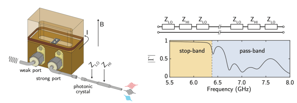
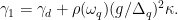


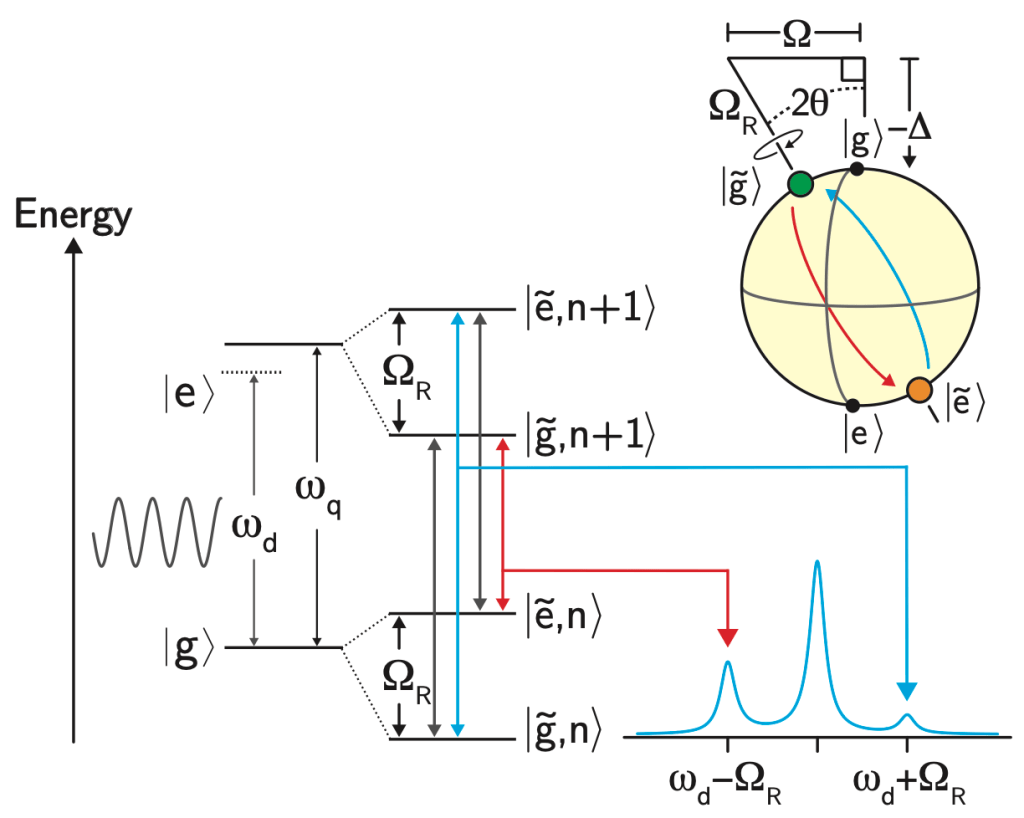
 . Due to the shaped loss spectrum, the area of one sideband can be supressed, indicating that the qubit will emit radiation at this frequency at a lower rate compared to the other sideband. Top right: under the presence of the drive, the quantization axis of the qubit also rotates, which changes which qubit states can be prepared/stabilized.


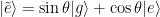


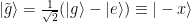


![\dot{\rho} = i[\rho,H] + \gamma_0 \cos{(\theta)}\sin{(\theta)}\mathcal{D}[\tilde{\sigma}_z]\rho + \gamma_{-} \sin{^4\left(\theta\right)} \mathcal{D}[\tilde{\sigma}_{+}\rho + \gamma_{+}\cos{^4\left(\theta\right)} \mathcal{D}[\tilde{\sigma}_{-}]\rho.](https://s0.wp.com/latex.php?latex=%5Cdot%7B%5Crho%7D+%3D+i%5B%5Crho%2CH%5D+%2B+%5Cgamma_0+%5Ccos%7B%28%5Ctheta%29%7D%5Csin%7B%28%5Ctheta%29%7D%5Cmathcal%7BD%7D%5B%5Ctilde%7B%5Csigma%7D_z%5D%5Crho+%2B+%5Cgamma_%7B-%7D+%5Csin%7B%5E4%5Cleft%28%5Ctheta%5Cright%29%7D+%5Cmathcal%7BD%7D%5B%5Ctilde%7B%5Csigma%7D_%7B%2B%7D%5Crho+%2B+%5Cgamma_%7B%2B%7D%5Ccos%7B%5E4%5Cleft%28%5Ctheta%5Cright%29%7D+%5Cmathcal%7BD%7D%5B%5Ctilde%7B%5Csigma%7D_%7B-%7D%5D%5Crho.&bg=ffffff&fg=010101&s=0&c=20201002)

![\mathcal{D}[A]\rho = \left( 2 A \rho A^{\dagger} - A^{\dagger}A\rho - \rho A^{\dagger}A\right)/2](https://s0.wp.com/latex.php?latex=%5Cmathcal%7BD%7D%5BA%5D%5Crho+%3D+%5Cleft%28+2+A+%5Crho+A%5E%7B%5Cdagger%7D+-+A%5E%7B%5Cdagger%7DA%5Crho+-+%5Crho+A%5E%7B%5Cdagger%7DA%5Cright%29%2F2&bg=ffffff&fg=010101&s=0&c=20201002)


 )
)
 oscillator with superconducting materials. The key element of this circuit is a Josephson junction, which is made of aluminum oxide sandwiched between layers of superconducting aluminum. The junction acts as a nonlinear inductor that modifies the energy level spacing of the
  ) and excited (
 ). The two levels form a quantum bit (qubit). The qubit is designed to be tunable in frequency by placing two Josephson junctions in a parallel with each other. By applying a magnetic field using a wire carrying current, a magnetic flux is threaded through the loop to change the qubit frequency.
 apart. To couple the qubit and mechanical oscillators, the authors use the piezoelectricy of the lithium niobate film. The mechanical motion of this material produces an accumulation of electric charges onto aluminum pads located on both chips, which are designed to be the capacitive element of the qubit. The qubit capacitor is charged by the motion of the mechanical oscillators, ensuring that the two systems are linked together.
 ). Note that the mechanical frequencies of the two oscillators are different, so the qubit can only be in resonance with one at a time. This allows for the direct exchange of energy between qubit and either oscillator at a rate related to the capacitive coupling between the two,
  9.5 MHz,
  10.5 MHz. The Hamiltonian that describes the interaction between a qubit and mechanical oscillator on resonance the Jaynes-Cummings interaction:
 and
and  are the creation, annihilation operators for the mechanical oscillator and qubit respectively. When on resonance, the qubit and mechanical oscillator swap their respective states in time
  24-26
24-26  depending on the particular oscillator.
 and
and  where
where  represents the state of the mechanics and the qubit. In between a full swap, the qubit and mechanical oscillators are entangled together with the joint state
  .
. , or
, or  state. The joint state
  , describe the phonon number of a particular mechanical oscillator,
  …, and whether the qubit is in the ground or excited state,
  . The qubit frequency is tuned to be on resonance with either mechanical mode for a time corresponding to a full swap. When the swap operation is applied to the joint state
  , the system remains unchanged since both subsystems are in their ground state and there is no energy to exchange. Under the swap, the state
  . The mechanical oscillator is now in a superposition state, but the state of the mechanical oscillator is not entangled with the qubit state.
 , is now set by the direct capactive coupling,
  , the detuning between qubit and mechanics,
  , and other qubit parameters. In the limit that the detuning between qubit and mechanics is larger than the the capacitive interaction rate (
 ), the interaction shown in
 is the operator version of the number of phonons,
  , in the mechanical oscillator.
  , where
  . By comparing the combined Hamiltonian with the one of just the qubit, we see that the effect of the interaction is to modify the transition frequency of the qubit (represented by everything before the
  ). For every additional phonon in the mechanical oscillator, the qubit transition frequency shifts by
  and allowed to precess for a variable time,
  . During this time, the superposition state accumulates a phase at rate
  for two phonons, and so on. The phase accumulated then reflects the probability (
 ) that the mechanical oscillator contained zero, one, two, etc… phonons. The qubit state evolves to
  , where the phase accumulated is
  . The authors rotate the qubit back into its measurement basis and monitor the final population of the qubit excited state as a function of the interaction time,
 ![S(t) = \sum_n A_n e^{-\kappa t/2} \cos [(2 n \chi t) + \phi_n]](https://s0.wp.com/latex.php?latex=S%28t%29+%3D+%5Csum_n+A_n+e%5E%7B-%5Ckappa+t%2F2%7D+%5Ccos+%5B%282+n+%5Cchi+t%29+%2B+%5Cphi_n%5D&bg=ffffff&fg=010101&s=0&c=20201002)
 . It also includes a number dependent phase offset,
  , and the phonon decay constant,
  . This captures the dynamics of the qubit trajectory even when the phonon probabilities are changing due to energy decay. The figure below shows an interferometry trace and the fit used to extract the phonon population in the mechanical oscillator. The trace contains a combination of various frequency oscillations each corresponding to a different phonon number. The weight of a particular frequency in the combination represents the probability of the corresponding phonon number to be present in the mechanical state being measured.
 , where the mechanical oscillators can contain
  phonons, and the qubit can be in either the ground (
 ) state. First the qubit is prepared in its excited state with
  . A half swap between the qubit and the first mechanical oscillator entangles the two,
  . This is accomplished by bringing the qubit into resonance with the mechanical oscillator for only half the time required the perform a full swap as seen in
  . This leaves the qubit in the ground state with the two mechanical state fully entangled together
  .
.
 , and the second term describes the qubit as a two level system with transition frequency
  and
and  conserve total excitation number, we can think of this interaction term as the qubit and the resonator “trading” excitations with a rate
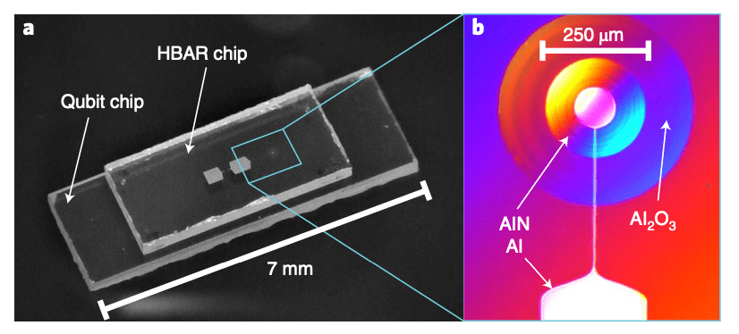
 . This can be used as a tool to measure how long phonons will remain in the HBAR device by first promoting the qubit to its excited state and then shifting the qubit’s frequency so that it’s resonant frequency is the same as that of the mechanical mode for a time
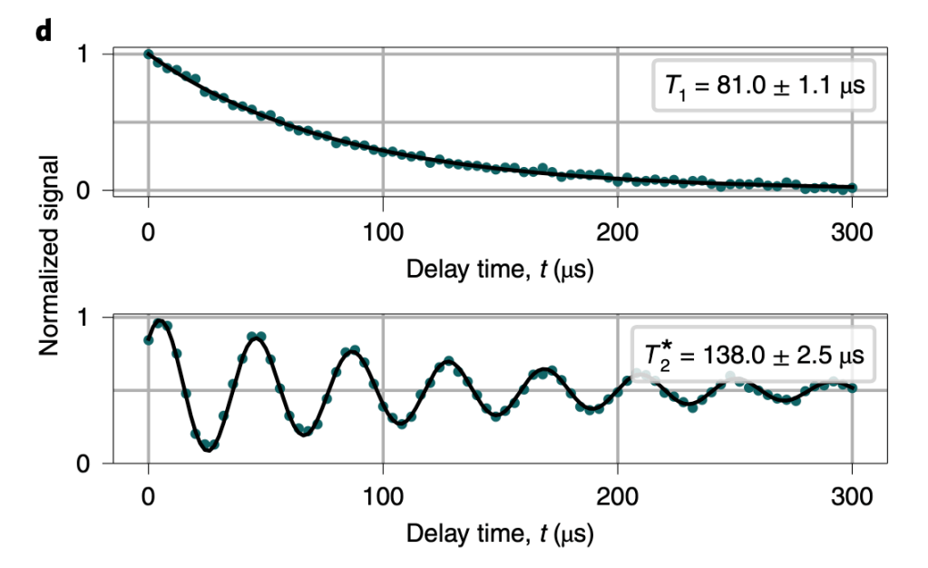

 , which is found to be
  , where the mean phonon number
  has been introduced. This is simply a Poisson distribution in phonon number, and interestingly by measuring the mean phonon number it’s possible to learn about the quantum mechanical fluctuations in the phonon resonator!
 is the difference in resonant frequency between the qubit and mechanical mode) is much larger than the coupling rate,
  can be approximated as:
 has been introduced. Writing the system Hamiltonian down in this from is typically called the dispersive regime, and this allows us to see that the effective qubit frequency
 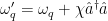 is now shifted by the number of excitations in the mechanical resonator! Oftentimes, in order to investigate the dispersive interaction between a qubit and a resonator, the authors will measure the qubit’s absorption spectrum, which is the frequency at which the qubit absorbs energy and is driven from its ground to excited state. This is also often called the qubit spectrum. If the qubit and resonator both have extremely low loss (both loss rates must be much less than
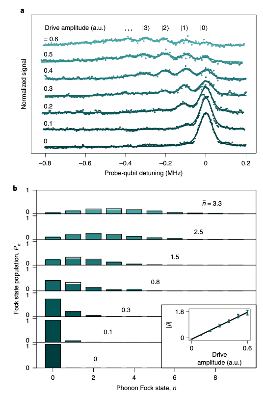
 . As a function of time, the qubit will accumulate a phase on the component of its wavefunction corresponding to the excited state of:
  , where
  is the number of excitations in the HBAR device. It’s important to note here that because the HBAR is in a Fock state, there is not a distribution of phonon numbers now as there would be for a coherent state, but rather one single Fock state describes the quantum state of the HBAR! After allowing the qubit state to accumulate phase for some amount of time, the qubit’s state is then rotated with the same phase as the pulse that prepared the original superposition state. This means that if the qubit accumulated no extra phase, it would be repositioned to the excited state (assuming that there are no losses). In reality the probability of measuring the qubit in its excited state will always decay in time, but the presence of phonons in the HBAR device can be measured from the frequency of oscillation from this measurement. The frequency of oscillation can be calculated to be equal to
  , where
  is the phonon number in the HBAR resonator. Fig. 4 details this measurement as a function of time for several different swap operations. At a time of approximately
  , which corresponds to the time
  , the authors are able to tell whether or not the resonator has an odd or even number of phonons based on whether or not the Ramsey decay is at a maximum or minimum! At this time, if there are an even number of phonons in the HBAR, the qubit phase has accumulated an even integer multiple of
  so that qubit superposition states are re projected to the excited state prior to measurement. Similarly, an odd number of phonons in the HBAR results in an odd multiple of
 , the authors are able to determine the parity (even-ness or odd-ness) of the phonon number in the HBAR resonator. (c) Comparison of measured parity based on two measurement schemes described by spectroscopic measurements (panel (a)), as well as measured parity by Ramsey measurements (panel (b)), the authors find very good agreement in measured parity between the two measurement schemes!

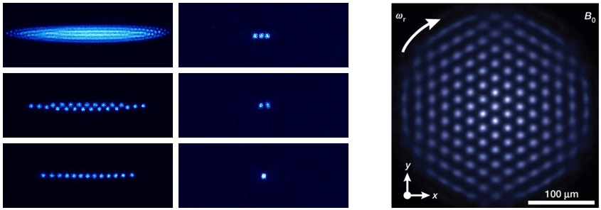

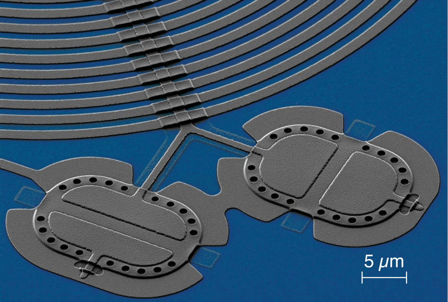

 circuit, which oscillates at a resonant frequency given by
  . The
. The  for the
  and
and  for the two drums. Then a quantum measurement of drum
  ‘s position is given by
  ,
, .
. , where
  is the average number of microwave-frequency photons inside the circuit. The drum energies are given by
  , where
  is the average number of phonons in drum
 photons. The lower-frequency drums are more occupied with
  phonons in each drum. With careful engineering, the authors can control and measure the two-drum system with single-phonon level precision.
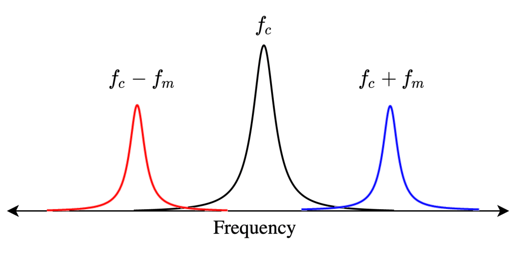
 , and blue sideband at
  .
. by exactly the mechanical frequency
  of the oscillators (see image above). We call the peak at
  the red sideband, and the peak at
  the blue sideband. By sending a sequence of microwave pulses at these sideband frequencies, the authors are able to initialize, entangle, and readout the motional states of the two drums.
 coupled to an LC circuit
  .
. and vice versa. For example, when applied to the state
  (1 phonon, 0 photons), for a time
  , the resulting evolution gives
  . If a blue sideband pulse is applied, the interaction is very different :
 , the resulting state takes the form (no normalization for simplicity)
  , where
  is the probability of generating an entangled pair.
 ,
,  ,
,  , and
, and  .
. to maximize the fidelity of the entanglement protocol. A red sideband pulse can be used to cool the drums to their quantum ground state. Due to the swap interaction described above, a phonon of energy in the drum is converted into a photon of energy in the LC circuit. If the decay rate of the circuit is fast enough (which it is in this experiment), the converted photon is emitted out of the circuit before it can be swapped back into the drum. If the pulse is applied for a long enough time, phonons are continually removed from the drum until there are nearly 0. This ground-state cooling technique was first demonstrated in macroscopic objects 10 years ago, using
  refer to the cosine and sine components of the signal:
 represents one quadrature,
  represents the other. In a blue sideband measurement,
 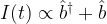 is proportional to position fluctuations and
  is proportional to momentum fluctuations. The authors send in a blue sideband pulse and look at the reflected I and Q signals to extract the position and momentum of each drum. These I and Q measurements can be done relatively easily using standard microwave electronics.
 , and plot the results. To show how the position and momentum of the drums are correlated, the authors plot each data point in phase space where the
  axes represent different combinations of
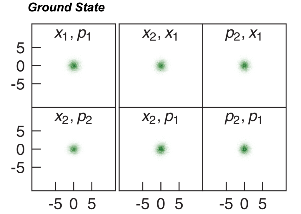
 and
and  phonons respectively, which indicates that the ground-state cooling is pretty successful.
 and
and  are clearly correlated, while momenta
  and
and  are clearly anti-correlated. This is a remarkable result as the two drums are physically separated and yet are moving in a coordinated way.
 , with elements defined by
 can represent
 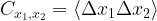 . If two variables, say
  . If they are correlated, then
  will have some nonzero value.
 of the partial transpose of the covariance matrix satisfies
  , then the two-drum mechanical state is entangled. Covariance matrices for the two cases are shown below:
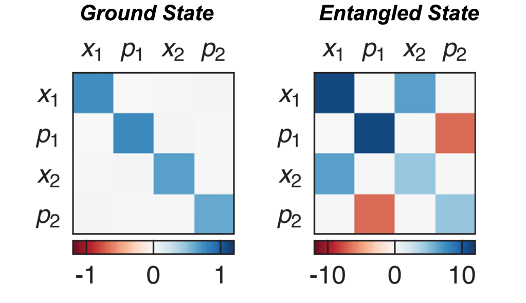
 and
and  creates off-diagonal elements in the covariance matrix. The authors find that by varying the entangling pulse time, the value of
  , verifying quantum entanglement for long enough entangling pulses. At the longest entangling time measured,
  to reflect only position/momentum fluctuations, without any additional unwanted fluctuations. In practice, however, the I and Q measurements also contain vacuum noise, so that the position/momentum measurements take the form
 ,
, 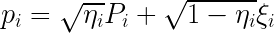
 ,
,  are the true values of position/momentum,
  is the vacuum noise of each I/Q measurement (basically just a random variable with variance 1/2), and
  is the measurement efficiency. If the value of
  is small enough, then the measurements of
 is the geometric mean of the efficiencies. The smaller the value of
  is to
is to  threshold. The authors show the calculated value of
  as a function of entangling pulse time:
 (left) and extracted true values of
  indicates the threshold for quantum entanglement.
 . The wavelength of light at these frequencies is given by
  for a signal with frequency 5 GHz. This means that the structures which couple our qubits together must be (of order) this size and are much larger than the qubits themselves! For a simple case, like coupling two qubits together this does not present any challenges[2], but as superconducting processors become larger in quantum volume (and therefore spatial size), it becomes more and more important to think critically about how we can create a smaller spatial structure with which to couple two or more qubits.
 , which is approximately 5 orders of magnitude smaller than the wavelength of a signal which travels at the speed of light! SAW devices are created by fabricating metal strips called interdigitated transducers (IDT for short) on a piezoelectric substrate. In a piezoelectric material, the electric fields in the material induce mechanical strain and vice versa so that an AC voltage applied across the metal strips launches a strain wave propagating across the substrate at the same frequency (see Fig. 1 for a schematic). Here, the wavelength of the surface wave is defined by the periodicity of the metal finger structure, so we are able to create high frequency resonators using standard nano-fabrication techniques.

 is very common for these types of experiments). The chip containing the SAW resonator is then fastened on top of the substrate where the qubit is fabricated. Using an experimental setup like this also allows one to tune the coupling between the qubit and SAW via on-chip inductors, which can allow us to study each system independent from one another. By coupling the qubit to a SAW device, we can transfer excitations from the qubit to the SAW (and vice versa). For example, one can often write the interaction between the SAW and the qubit to be:
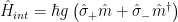
 are the creation and destruction operators for excitations in the qubit, and
  and
and  are bosonic operators for the phonon modes in the SAW. If we prepare the qubit in the excited state and have no phonons in the SAW resonator, then after a time
  , the excitation will be transferred to the SAW! As an equation:
 is the excited (ground) state of the qubit and the number in the state vector denotes the number of phonons excited in the SAW device.
 , the control lines
  control the state of that qubit and the control line labeled
  controls the local magnetic field which tunes the resonant frequency of that qubit. The coupler labeled
  controls the coupling to the acoustic channel on a separate chip, and the control line
  allows for the control of the coupling strength via an external magnetic flux.
 measurement is performed, where the qubit is put into its excited state via a microwave pulse, and then the probability of the qubit remaining in its excited state as a function of time is measured. The result is shown in Fig. 4.
 s. This is because the qubit excitation is lost to a phonon, and the phonon travels to the other end of the phonon channel, then it is reflected back to the original SAW where it is in turn converted back to a qubit excitation! A similar, yet weaker feature is also noticeable near 2
 prepares qubit 1 into its excited state. Then the coupling between the acoustic channel and qubit 1 is turned on (represented by
  ). After a set amount of time, the coupler between the acoustic channel and qubit 2 is turned on (represented by
  ), and the state of qubit 2 is measured.
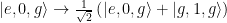
 , where the first index denotes the state of qubit 1,
  represents the number of phonons in the acoustic channel, and the final index labels the state of qubit 2. Upon the arrival of the phonon on the other side of the channel, the authors turn coupler 2 on and “catch” the traveling phonon so that the total process is:
 , as well as factored out the index which denotes the phonon number. Because we can factor out the phonon number here, we can write the two qubit wavefunction after this process as
  , which we recognize to be a Bell state, which is entangled! Results from this experimental protocol are shown in Fig. 6a. Additionally, a reconstruction of the two qubit density matrix allows the authors to verify that the state they have prepared is actually a Bell state! See Fig. 6b for a comparison with theory.
 ). Here, we say that Q1 probes the state of Q2 via phonons.
 . Experimentally, the phase
  radians about the x-axis of the Bloch sphere and measure the state of qubit Q2. As we sweep the phase of the first pulse, we should expect an oscillation in the excited state probability of qubit Q2. As a contrast, they repeat the measurement where the only change is they have first excited qubit Q1 and turned on the relevant couplers. If a phonon is released via qubit Q1, this will again manifest as a phase change relative to the first measurement. The relevant pulse sequence and results are shown in Fig. 8.
 . This means that they can use the phonon channel to perform phase sensitive measurements of “arbitrary” quantum systems (where of course here that system is another qubit)!
 , and a partition in the centre of the box. A small demon stands by a massless door in the partition, and strategically opens the door so that all the particles pass into one half of the box, and the other half of the box is a vacuum. Maxwell intended his demon to challenge the interpretation of the Second Law: without doing any work, the demon has lowered the entropy of the box. However, it can be understood in a different way: the demon is only able to change the system’s entropy via possession of information about the particles – i.e. their position and momentum. Therefore, information can be used to perform more work than expected by the Second Law. This understanding led to the famous slogan“information is physical” [2] – meaning it has to be accounted for in thermodynamics.
 is the Helmholtz energy, describing the maximum extractable work,
  the internal energy of the system,
  the actual extracted work, and
  the entropy production during the process in which work is extracted. We can see from this relation that when entropy increases,
  , the extracted work is smaller than the maximum extractable work. But when entropy decreases,
  – i.e. because of a quantum non-Markovian process – the extracted work is higher than the maximum.
 ) and cold (
 ) reservoirs.
 and
and  , as in the above image. It absorbs an amount of heat
  from the hot reservoir, performs an amount of work
  , and rejects an amount of heat
  to the cold reservoir. During the most efficient possible process – the Carnot cycle, which is reversible and generates no entropy – the efficiency of the engine is
 , the efficiency is
 . The goal now is to determine a similar expression for a corresponding quantum engine, which may well have
  .
. and the irreversible work
  . The reversible work is
 is the Helmholtz energy of the equilibrium state – essentially, the work that can be extracted from the system after it has reached thermal equilibrium with its environment –
 is the relative von Neumann entropy between the state of the system at time
  and the equilibrium state
  . Relative entropy is a measure of how much information is shared between two quantum states – how easy it is to distinguish the two states, so
  tells us how far away
  is from the equilibrium state.
 positive when
  , which means it reduces the magnitude of the reversible work.
 . The density matrix is a much more general description of a quantum state, and describes systems which can lose information. When we are using the density matrix, expectation values of operators are found by taking the trace – for example, the energy expectation value is
 at time
  , and it interacts with a bath at temperature
  , according to Hamiltonian
  . After the system has evolved over a time
  , the state of the system is
  . The irreversible work after this time is
![\Delta W_{\rm irr} = k T [S(\rho_0 || \rho_{\infty}) - S(\rho_t || \rho_{\infty})].](https://s0.wp.com/latex.php?latex=%5CDelta+W_%7B%5Crm+irr%7D+%3D+k+T+%5BS%28%5Crho_0+%7C%7C+%5Crho_%7B%5Cinfty%7D%29+-+S%28%5Crho_t+%7C%7C+%5Crho_%7B%5Cinfty%7D%29%5D.+&bg=ffffff&fg=010101&s=1&c=20201002)
 and
and  . It is worth noting that the information lost during an open quantum system evolution is usually information about the coherence – i.e. which superpositions the initial state contained.
 , until it is in state
  . The interaction is described by the Hamiltonian
  . The change in the system’s energy expectation value over the interaction is equivalent to the amount of heat it absorbs:
 ![\Delta Q_h ={\rm Tr}[H_0(\rho_0) - {\rm Tr}[H_0(\rho_1)]= {\rm Tr}[H_0(\rho_0 - \rho_1)]](https://s0.wp.com/latex.php?latex=%5CDelta+Q_h+%3D%7B%5Crm+Tr%7D%5BH_0%28%5Crho_0%29+-+%7B%5Crm+Tr%7D%5BH_0%28%5Crho_1%29%5D%3D+%7B%5Crm+Tr%7D%5BH_0%28%5Crho_0+-+%5Crho_1%29%5D&bg=ffffff&fg=010101&s=1&c=20201002) . The entropy of the system changes by
. The entropy of the system changes by  , which has a contribution from the heat absorption,
  , and a contribution from the evolution of the state of the system:
 . No entropy is produced.
![\Delta Q_c = {\rm Tr}[H_1(\rho_0 - \rho_1)]](https://s0.wp.com/latex.php?latex=%5CDelta+Q_c+%3D+%7B%5Crm+Tr%7D%5BH_1%28%5Crho_0+-+%5Crho_1%29%5D&bg=ffffff&fg=010101&s=1&c=20201002) . The entropy of the system changes by
. The entropy of the system changes by  , which – just like in Step 1 – has a contribution from the heat rejection, and a contribution from the evolution of the state of the system.
 . The irreversible work is
 , and then
  . Therefore, non-Markovian dynamics can be used to construct engines which are more efficient than a Carnot engine.
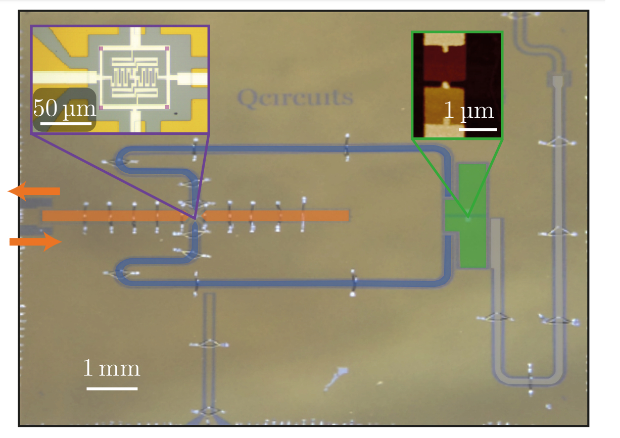
 photons in only
  measurements. Finally, I discuss the potential applications of the device and protocol developed in this work.

 . The buffer cavity is strongly coupled to the transmission line in order to capture the traveling wavepacket and temporarily hold it, making it a stationary mode. Resolving the number of photons in the signal requires enough time to make the measurements, however the strong coupling between the transmission line and buffer cavity, used to capture the wavepacket, results in the signal quickly leaking out of the stationary mode and back into the propagating line. To ensure there is enough time to measure the photon number, the state is swapped into a long lived memory cavity that can store the signal while it is being read out. This is done using a Josephson ring modulator (JRM), which swaps the states of the buffer and memory cavities. Once the state has been transferred into the memory, a qubit and readout system can be used to determine the number of photons present. After measuring the state, the JRM swaps the state back into the buffer where is it quickly emitted into the transmission line. This resets the system and allows for the next operation to proceed.
 GHz) and memory (
 GHz) cavities frequencies. This provides the energy required to transfer a state from the buffer to the memory cavity. The pump enables a beam splitter interaction between the buffer and memory, described by the Hamiltonian shown in
  (Equation 1)
 is the pulse shape of the pump,
  is the annihilation operator of the buffer mode, and
  is the creation operator for the memory mode. When the pump is on, the state present in the buffer mode is swapped into the memory at a rate
  , the buffer will contain 0 photons and the memory will have 1 photon. The authors use this interaction to move the wavepacket from the buffer cavity to the memory for measurement. This process can also be used in reverse; a photon contained in the memory cavity can be transferred into the buffer by applying the same pump. The authors use this interaction to reset the device by emptying out the memory cavity. The pump is turned on to swap the memory state into the buffer, where the wavepacket quickly escapes into the transmission line.
 bit determines if
  is included in that sum. For example,
  , so for 13, bit 0 = 1, bit 1 = 1, bit 2 = 1, and bit 3 = 1. Here, the qubit state after each measurement (either g or e) represents the value of the bit being measured (which can be either 0 or 1). Each photon number is then identified as a unique series of g’s and e’s (or 0’s and 1’s). In this work, the authors measure wavepackets that contain up to 3 photons, using two measurements to distinguish between 0, 1, 2, and 3 photons as shown in
  and
and  .
. (Equation 2)
 , where
  . The combination
  is the operator version of the number of photons, n, in the memory cavity. By comparing the total Hamiltonian with the one of just the qubit, we see that the effect of the interaction is to modify the transition frequency of the qubit (represented by everything before the
  ). So now, the qubit transition frequency is dependent on the number of photons in the memory cavity (
 ). For every additional photon in the memory cavity, the qubit transition frequency shifts by
  using a
  , the qubit state acquires a phase that is proportional to the number of photons,
  . The qubit is then projected back onto the z-axis using a second
  so that when the photon number is even the phase acquired is an even multiple of
  with
with  . Since the qubit state remains
  after the interaction, the qubit ends up back in the ground state. If there are an odd number of photons in the memory (1 or 3), the qubit phase is
  ,
,  . The qubit state is
  . The second
  to distinguish between 0 and 2 photons (or 1 and 3 photons), the 1st bit of information. The axis of the second
  relative to the original axis. If there is 1 memory photon, the qubit ends in the ground state and if there are 3 photons, the qubit is excited.
 can be represented by only
  bits. Since it takes only one measurement per bit, large numbers of photons up to
  measurements. This provides a way to efficiently measure lots of information encoded in quantum states with many photons.


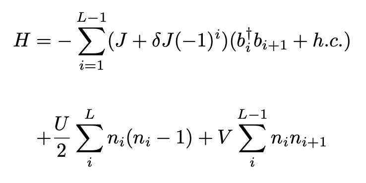
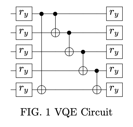

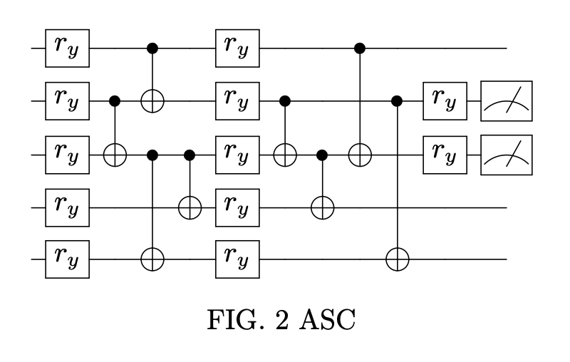

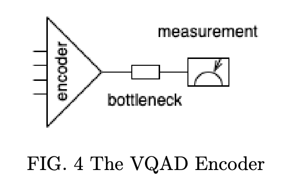


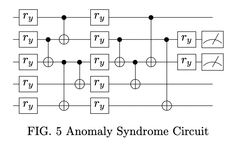

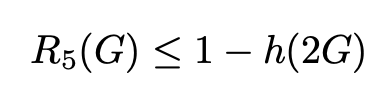

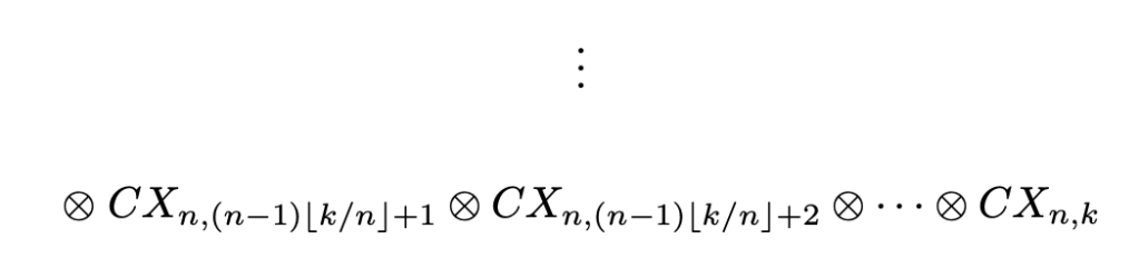
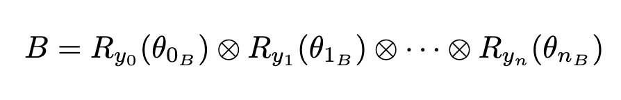


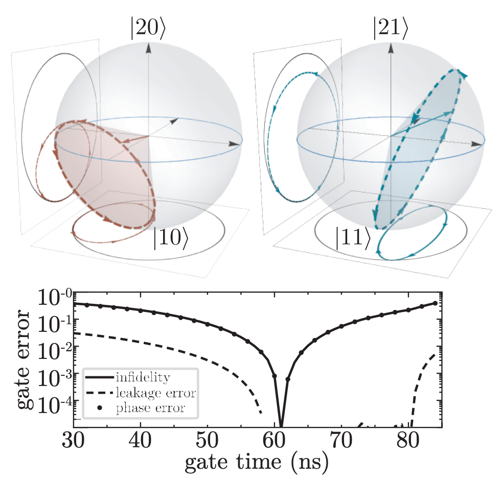
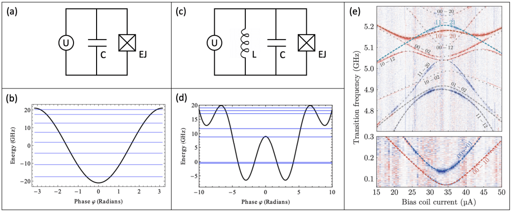
 up to 500
 s [
s [ , where
  and
and  are the amount of charge across the Josephson junctions in each circuit. The capacitive coupling produces little effect on the computational states
  , since transition matrix elements of
  and
and  states will also remain unaffected due to parity selection rules. The states that will be affected are the higher energy non-computational states
  and
and  which have higher transition frequencies, meaning the
  (see Fig. 2b). This level repulsion becomes key in connecting the two fluxonium subspaces, inducing an on-demand qubit-qubit interaction.
 and
and  , which are detuned by
  and
and  caused by the
  coupling.
 and
and  . If the gate pulse is applied over a short duration, one will have unwanted leakage to the nearby transition. Although the prospect of a CZ gate between fluxoniums is attractive, for the device parameters used in this work,
  at the transition frequency
  , we will observe Rabi oscillations between the
  , the circle traced by the Bloch vector shifts such that it doesn’t make it all the way to the excited state (a review of Rabi oscillations can be found
  transitions,
 is detuned from
  such that full Rabi oscillations for both transitions are completed in the same amount of time. (b) Cones traced by each state vector on the Bloch sphere due to the applied Rabi drive tone,
  from
from  rotation on both states simultaneously, but how does this help us perform a selective CZ gate on just
  and
and  , corresponding to a “geometric phase” accumulation
  for each system (you can read more about geometric phase
  to the states. This is effectively the same as assigning a phase difference
  between two trajectories to realize a control-Phase operation (again, you can review quantum logic gates
  !
!  if a control-Phase operation is also applied! In this work, the theory is verified by simulation of the complete system hamiltonian and verified by experiment! The authors state that this procedure can readily be extended to any other phase accumulation, an exciting result that can be further studied in other systems.
 s : 61 ns) is unmatched across quantum computing platforms (to the best of the authors’ knowledge).