Quantum Communication with itinerant surface acoustic wave phonons

Authors: E. Dumur, K.J. Satzinger, G.A. Peairs, M-H. Chou, A. Bienfait, H.-S. Chang, C.R. Conner, J. Grebel, R.G. Povey, Y.P. Zhong, A.N. Cleland

First Author’s Primary Affiliation: Pritzker School of Molecular Engineering, University of Chicago, Chicago, IL 60637, USA

Manuscript: Published in NPJ Quantum Information

Introduction

Superconducting qubits are among the state of the art architectures in the development of quantum processors. In order to successfully build a functioning quantum computer, it is essential to be able to transfer information about quantum states amongst multiple qubits while maintaining the “quantum” properties of these states. Typically, one would couple two or more superconducting qubits via a transmission line where the signal travels at the speed of light. Importantly, because superconducting qubits operate in the GHz frequency range, the wavelength of light with this frequency is large relative to the size of the qubit, which is approximately $(1mm)^{2}$ . The wavelength of light at these frequencies is given by $\lambda = 6 \textrm{cm}$ for a signal with frequency 5 GHz. This means that the structures which couple our qubits together must be (of order) this size and are much larger than the qubits themselves! For a simple case, like coupling two qubits together this does not present any challenges[2], but as superconducting processors become larger in quantum volume (and therefore spatial size), it becomes more and more important to think critically about how we can create a smaller spatial structure with which to couple two or more qubits.

Surface acoustic wave (SAW) devices utilize the “slow” speed of surface sound waves in crystals (typically about 4000 m/s) in order to create high frequency resonant structures with a small spatial footprint. For example, in order to create a structure with a resonant frequency of 4 GHz, one would need a wavelength of $\lambda = (4000 \textrm{m/s})/(4\textrm{GHz}) = 1 \mu \textrm{m}$ , which is approximately 5 orders of magnitude smaller than the wavelength of a signal which travels at the speed of light! SAW devices are created by fabricating metal strips called interdigitated transducers (IDT for short) on a piezoelectric substrate. In a piezoelectric material, the electric fields in the material induce mechanical strain and vice versa so that an AC voltage applied across the metal strips launches a strain wave propagating across the substrate at the same frequency (see Fig. 1 for a schematic). Here, the wavelength of the surface wave is defined by the periodicity of the metal finger structure, so we are able to create high frequency resonators using standard nano-fabrication techniques.

FIg. 1
Schematic of an IDT structure (red) which is driven by an AC voltage and launches surface acoustic waves (green)

In addition to using IDT structures to launch SAWs, we can also add periodic metallized structures on either side of the IDT launcher which act to reflect phonons emitted from the IDT (called mirrors). See Fig. 2 (adapted from [3]) for a schematic which details both the IDT as well as the mirror structures.

Figure 2 Schematic of a SAW resonator which contains both the IDT which launches SAWs (center), and the mirrors on either side of the IDT which form an *acoustic* cavity.

Together, the IDT and mirror structure create an acoustic cavity for phonons, where the spatial size is much smaller than a cavity for microwave photons at the same frequency!
GHz-frequency SAW resonators have been coupled to superconducting qubits before, sometimes in a “flip-chip” configuration[4]. This allows the experimentalist to fabricate a standard superconducting qubit on one substrate (typically on silicon or sapphire) and the SAW resonator on a separate piezoelectric substrate (LiNbO $_3$ is very common for these types of experiments). The chip containing the SAW resonator is then fastened on top of the substrate where the qubit is fabricated. Using an experimental setup like this also allows one to tune the coupling between the qubit and SAW via on-chip inductors, which can allow us to study each system independent from one another. By coupling the qubit to a SAW device, we can transfer excitations from the qubit to the SAW (and vice versa). For example, one can often write the interaction between the SAW and the qubit to be:

$\hat{H}_{int} = \hbar g\left(\hat{\sigma}_{+} \hat{m} + \hat{\sigma}_{-} \hat{m}^{\dagger} \right)$

Here, ${\sigma}_{\pm}$ are the creation and destruction operators for excitations in the qubit, and $\hat{m}$ and $\hat{m}^{\dagger}$ are bosonic operators for the phonon modes in the SAW. If we prepare the qubit in the excited state and have no phonons in the SAW resonator, then after a time $\pi/g$ , the excitation will be transferred to the SAW! As an equation:

$|e,0\rangle \rightarrow |g,1\rangle$

Here the quantum state is written as a product of both the qubit state and the state of the SAW, where $|e(g)\rangle$ is the excited (ground) state of the qubit and the number in the state vector denotes the number of phonons excited in the SAW device.

Experimental Details and Preliminary Results

In this set of experiments, the primary goal is to use two SAW resonators to mediate the quantum state transfer between two qubits which are separated spatially by using a phonon based communication channel. Here, the previously mentioned flip-chip configuration will be used. On the sapphire substrate, the two qubits are fabricated. Each qubit contains a SQUID loop, which means that the resonant freuquency of the qubit is tunable via an external magnetic flux threading the SQUID loop. Additionally extra control lines are added near each qubit which can manipulate the quantum state of the qubit. The control lines which manipulate the individual qubit states are known as XY lines, while control lines which provide local magnetic flux control to each qubit are known as Z lines. On the “top” LiNbO $_3$ chip, two IDT devices with the same resonant frequency (near 4GHz) are fabricated. These two IDT are separated by 2mm, which means it takes a phonon approximately 500ns to traverse from one IDT to the other. An acoustic mirror structure is added on one side of each IDT so that phonons are preferentially launched in one direction at certain frequencies (this specific design is called a unidirectional transducer, or UDT for short). This allows for constructive interference of phonons at some frequencies, which we will call the UDT regime. At all other frequencies phonons will not constructively interfere, and we will call this the IDT regime. Two tunable couplers are added on each chip so that the interaction strength between each qubit and each SAW resonator can be independently tuned. See Fig. 3 for a full schematic of the composite device.

Figure 3
(a) Schematic of the composite device and a description of each piece. (b) Effective circuit diagram which describes the circuitry necessary to manipulate the qubit states as well as couple the qubits to the acoustic resonators. For each qubit $Q_i$ , the control lines $Q_{xyi}$ control the state of that qubit and the control line labeled $Q_{zi}$ controls the local magnetic field which tunes the resonant frequency of that qubit. The coupler labeled $G_i$ controls the coupling to the acoustic channel on a separate chip, and the control line $G_{zi}$ allows for the control of the coupling strength via an external magnetic flux.

Figure 3
(a) Schematic of the composite device and a description of each piece. (b) Effective circuit diagram which describes the circuitry necessary to manipulate the qubit states as well as couple the qubits to the acoustic resonators. For each qubit $Q_i$ , the control lines $Q_{xyi}$ control the state of that qubit and the control line labeled $Q_{zi}$ controls the local magnetic field which tunes the resonant frequency of that qubit. The coupler labeled $G_i$ controls the coupling to the acoustic channel on a separate chip, and the control line $G_{zi}$ allows for the control of the coupling strength via an external magnetic flux.

The first experiment that can be done with this device is the independent characterization of a single qubit, for example qubit Q1, when it is weakly coupled to the phononic quantum channel. This characterization allows the authors to verify that the qubits have long enough coherence to take full advantage of the communication channel. This means that we need the qubit to maintain its state much longer than the phonon travel time of 500ns, otherwise we won’t be able to measure any effects due to phonons traversing the communication channel! In order to measure how long the qubit can maintain its state, a T $_1$ measurement is performed, where the qubit is put into its excited state via a microwave pulse, and then the probability of the qubit remaining in its excited state as a function of time is measured. The result is shown in Fig. 4.

Figure 4
T $_1$ data for qubit Q1 across a broad range of qubit frequencies. Interestingly, we see that when the qubit is near-resonant with the SAW device, its lifetime drops dramatically!

At first glance, many striking features of this measurement are apparent. First, over the frequency range of approximately 3.85GHz to 4.15GHz, the qubit does not remain in its excited state for very long. This is because over this frequency range, the SAW resonator has a high conductance, and therefore the qubit excitation is transferred into a phonon. Finally, and perhaps most interestingly, in the range where the qubit excitation is lost to a phonon, the qubit excited state actually increases after roughly 1 $\mu$ s. This is because the qubit excitation is lost to a phonon, and the phonon travels to the other end of the phonon channel, then it is reflected back to the original SAW where it is in turn converted back to a qubit excitation! A similar, yet weaker feature is also noticeable near 2 $\mu$ s. Because we can see these features, this is an indication that the qubit coherence is long enough such that we can use the full potential of the phonon communication channel in this device!
After significantly long coherence is verified, the authors attempt a quantum state transfer between the qubits. The experimental protocol is as follows: prepare qubit Q1 into its excited state, then turn on the coupling between qubit Q1 and a SAW resonator. This will allow for a phonon to be launched across the phonon channel. Then approximately 500ns later, the authors turn on the coupling between the other SAW resonator and qubit Q2. This will allow for the transiting phonon to be converted into an excitation in qubit Q2. The results are shown in Fig. 5.

Quantum state transfer in the UDT regime (left) and the IDT regime (right). We see that the state transfer is possible in both regimes, but much more effective in the UDT regime. The pulse sequence in the right panel demonstrates the measurement protocol: a pulse applied to qubit 1 via the control line $Q_{xy1}$ prepares qubit 1 into its excited state. Then the coupling between the acoustic channel and qubit 1 is turned on (represented by $K_1$ ). After a set amount of time, the coupler between the acoustic channel and qubit 2 is turned on (represented by $K_2$ ), and the state of qubit 2 is measured.

Quantum state transfer in the UDT regime (left) and the IDT regime (right). We see that the state transfer is possible in both regimes, but much more effective in the UDT regime. The pulse sequence in the right panel demonstrates the measurement protocol: a pulse applied to qubit 1 via the control line $Q_{xy1}$ prepares qubit 1 into its excited state. Then the coupling between the acoustic channel and qubit 1 is turned on (represented by $K_1$ ). After a set amount of time, the coupler between the acoustic channel and qubit 2 is turned on (represented by $K_2$ ), and the state of qubit 2 is measured.

Here we can see that when the SAW is operated in the UDT regime, the probability of Q2 being excited via a phonon is near 68%, while in the IDT regime it is much lower (only about 15%). This is an indication that operating in the UDT regime allows for highly efficient state transfer from one qubit to another mediated by phonons!!

Entanglement

Now that we know we can transfer a quantum state from one qubit to the other using phonons as an intermediate step, a logical next step is to attempt to create a non trivial multi-qubit state, specifically a Bell state! In order to do this experiment, the authors harness the utility of the tunable couplers mentioned previously. If we load an excitation into a qubit and turn on the coupling between the qubit and SAW resonator for a specific amount of time, the qubit excited state probability will decay to approximately 50% (see Fig. 6, approximately 175ns). At this time, there is a 50% chance the qubit has lost its excitation to the emission of a phonon in the communication channel, and we will call this launching “half” a phonon. Of course, we can write the process quantum mechanically:

$|e,0,g\rangle \rightarrow \frac{1}{\sqrt{2}}\left(|e,0,g \rangle+ |g,1,g\rangle\right)$

Here we have labeled the quantum states as the following $|Q1,\gamma,Q2\rangle$ , where the first index denotes the state of qubit 1, $\gamma$ represents the number of phonons in the acoustic channel, and the final index labels the state of qubit 2. Upon the arrival of the phonon on the other side of the channel, the authors turn coupler 2 on and “catch” the traveling phonon so that the total process is:

$|e,0,g\rangle \rightarrow \frac{1}{\sqrt{2}}\left(|e,0,g \rangle+ |g,1,g\rangle\right) \rightarrow \frac{1}{\sqrt{2}}\left(|e,g\rangle + e^{i\phi}|g,e\rangle\right)\otimes|0\rangle$

Here, we have introduced a relative phase difference $\phi$ , as well as factored out the index which denotes the phonon number. Because we can factor out the phonon number here, we can write the two qubit wavefunction after this process as $|\psi\rangle = \frac{1}{\sqrt{2}}\left(|e,g\rangle + e^{i\phi}|g,e\rangle\right)$ , which we recognize to be a Bell state, which is entangled! Results from this experimental protocol are shown in Fig. 6a. Additionally, a reconstruction of the two qubit density matrix allows the authors to verify that the state they have prepared is actually a Bell state! See Fig. 6b for a comparison with theory.

Figure 6
(a) Experimental results for the generation of the Bell state. We see that we have approximately 50% chance of measuring each qubit in its excited state. (b) A reconstruction of the two qubit density matrix. Here the red boxes represent the expectation for a perfect Bell state, and the dashed boxes are simulation results which take into account all of the losses in the system.

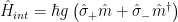
Phonon-Qubit Dispersive Interaction

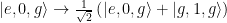
The final set of experiments performed with this remarkable device uses phonons as a probe of the state of one of the qubits. For example, the phase change of a phonon will be different if it interacts with a qubit in its excited state rather than its ground state. In order to test this, again the authors launch half a phonon using qubit Q1. When this phonon is traveling, the resonant frequency of qubit Q1 is changed so that the quantum state of Q1 is changed. When the phonon reaches qubit Q2, the coupler is turned on for a fixed amount of time (200 ns), and the phonon and qubit are allowed to interact. The phonon then reflects back to qubit Q1 and the coupler is turned back on so that the excitation is transferred back to Q1. If the phase of the qubit and the phase of the phonon interfere constructively, the qubit will return to its excited state. However, if they interfere destructively, the qubit will emit its remaining energy and relax to its ground state. Therefore, a measurement of the excited state probability of Q1 will tell us about the phase interference between the phonon and Q1! As we sweep the relative phase of Q1, we should expect to see oscillations in the excited state probability of Q1, where the peaks are constructive interference conditions and the valleys are destructive interference conditions. The relevant pulse sequences are shown in the right panel of Fig. 7.

Figure 7
A measurement of qubit Q1’s excited state probability as a function of its induced phase. There is a discrete phase change (salmon) when the qubit Q2 is prepared in its excited state prior to the measurement.

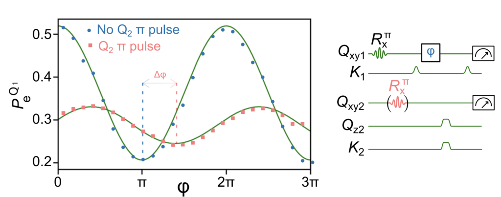
The experimental process can then be repeated, with the only difference being we have first excited qubit Q2 into its excited state, which means that the phonon should pick up an additional phase shift! This is read out as a discrete phase shift in the left panel of Fig. 7 (the salmon dots are shifted in phase relative to the blue dots by $\Delta\phi = 0.40\pi$ ). Here, we say that Q1 probes the state of Q2 via phonons.

Finally, the authors swap the roles of the two qubits and perform one final measurement. They prepare qubit Q2 in a superposition of its ground and excited states, with some variable phase $\theta$ . As an equation: $|\psi\rangle = \frac{1}{\sqrt{2}}\left(|g\rangle + e^{i\theta}|e\rangle\right)$ . Experimentally, the phase $\theta$ is set by the phase of a microwave pulse. Once the state is prepared, they wait a fixed amount of time and apply another pulse which rotates the state by $\pi/2$ radians about the x-axis of the Bloch sphere and measure the state of qubit Q2. As we sweep the phase of the first pulse, we should expect an oscillation in the excited state probability of qubit Q2. As a contrast, they repeat the measurement where the only change is they have first excited qubit Q1 and turned on the relevant couplers. If a phonon is released via qubit Q1, this will again manifest as a phase change relative to the first measurement. The relevant pulse sequence and results are shown in Fig. 8.

Figure 8
A measurement of qubit Q2’s excited state probability as a function of its induced phase via a microwave drive. There is a discrete phase change (salmon) when the qubit Q2 is prepared in its excited state prior to the measurement.

Again, there is a discrete phase shift in the excited state probability of qubit Q2, this time of $\Delta \theta = 0.95\pi$ . This means that they can use the phonon channel to perform phase sensitive measurements of “arbitrary” quantum systems (where of course here that system is another qubit)!

Conclusion

In conclusion, this remarkable set of experiments shows that it is possible to use a phonon-based communication channel to not only transfer a quantum state from one qubit to another, but it is also possible to perform more complex operations, such as preparing a two qubit Bell state! Finally, we can harness the power of traveling phonons to probe the characteristics of other quantum systems and learn about them by measuring a separate qubit!

References

[1] E. Dumur et al, npj Quantum Information 7, 1734 (2021)

[2] J. Majer et. a, Nature 449, 443–447 (2007)

[3] T. Aref et. al, Quantum acoustics with surface acoustic waves, in Super-
conducting Devices in Quantum Optics, edited by R. H. Hadfield and G. Johansson (Springer International Publishing, Cham, 2016) pp. 217–244.

[4] K. J. Satzinger et. al, Nature 563, 7733 (2018)

Many thanks to Piero Chiappina for his helpful comments, edits, and suggestions!