Quantum Entanglement of Macroscopic Mechanical Objects

Title: Direct observation of deterministic macroscopic entanglement

Authors: Shlomi Kotler, Gabriel A. Peterson, Ezad Shojaee, Florent Lecocq, Katarina Cicak, Alex Kwiatkowski, Shawn Geller, Scott Glancy, Emanuel Knill, Raymond W. Simmonds, José Aumentado, John D. Teufel

Institution: National Institute of Standards and Technology (NIST)

Manuscript: Published in Science, open access on arXiv

Quantum entanglement is one of the most bizarre and powerful phenomena in quantum mechanics. Over the years, physicists have created and observed entanglement of a wide range of systems, from the spin states of atoms to the polarization of photons. Most experiments to date, however, have studied quantum entanglement in the smallest of microscopic systems, the regime where quantum mechanics is most easily observed. It is much more difficult to observe quantum entanglement in macroscopic objects, where environmental disturbances seemingly destroy their quantum behavior. A recent paper from researchers at NIST reports observation of such entanglement: namely, the position and momentum of two physically separate mechanical oscillators. Entanglement of mechanical oscillators isn’t exactly new: position entanglement was first observed in the vibrational states of two atomic ions back in 2009. But this entanglement explores an entirely different regime, where the vibrations are not just of singular atoms, but the collective motion of billions of atoms in a macroscopic object.

SEM image of the two aluminum drums, and the complete LC circuit.

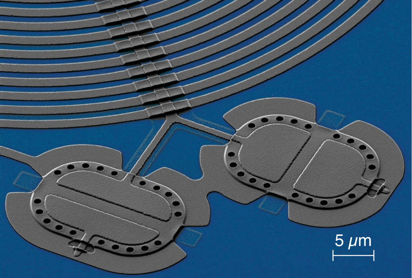
The study analyzes the mechanical oscillations of two drum-like membranes. The drums are patterned out of aluminum on a sapphire chip, are roughly 20 microns in length, and weigh roughly 70 picograms. While the drums are tiny to us- each drum is smaller than the width of a human hair- they contain several billion atoms, large enough to be considered ‘macroscopic’ for a quantum system. The membranes are designed to oscillate at 11MHz and 16MHz frequencies, respectively (they are purposefully designed to oscillate at different frequencies, so that each membrane can be identified). There is a metal base below each drumhead, so that the drumhead and the metal base act like a parallel-plate capacitor. When the drum vibrates, the distance between the plates changes, thereby changing the capacitance of the drum. By wiring up the drum to a large spiral inductor, we form an $LC$ circuit, which oscillates at a resonant frequency given by $1/\sqrt{LC}$ . The $LC$ circuit in this work is designed to oscillate at 6GHz. As the drum vibrates, the changing capacitance of the drum changes the resonant frequency of the $LC$ circuit. By probing the circuit frequency, we gain information about the motion of the drum. The device is placed inside a dilution refrigerator which cools the device down to temperatures below 10mK. At this temperature, aluminum becomes a superconductor and both the circuit and drums have very few energy loss mechanisms. Once energy enters either one of the cavities, it can remain for milliseconds. This gives the cavities narrow resonances in frequency space, making them well-suited to behave quantum mechanically.

Quantum Electromechanics- The Basics

We can measure the quantum properties of this electromechanical system by noting that both the microwave circuit and the mechanical drums are harmonic oscillators, which we can treat quantum mechanically with creation and annihilation operators: $\hat{a}$ for the $LC$ circuit, and $\hat{b}_1$ and $\hat{b}_2$ for the two drums. Then a quantum measurement of drum $i$ ‘s position is given by

$\hat{x}_i = x_{0, i}(\hat{b}^{\dagger}_i + \hat{b}_i)$ ,

and momentum by

$\hat{p}_i = ip_{0, i}(\hat{b}^{\dagger}_i - \hat{b}_i)$ .

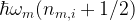
Quantum mechanically, the energies of these two oscillators are quantized. The average energy of the circuit is given by $\hbar\omega_c (n_c + 1/2)$ , where $n_c$ is the average number of microwave-frequency photons inside the circuit. The drum energies are given by $\hbar\omega_m (n_{m, i} + 1/2)$ , where $n_{m, i}$ is the average number of phonons in drum $i$ . Basic statistical mechanics tells us that the circuit and drums are naturally in a thermal state, with average photon/phonon numbers given by the Bose-Einstein occupation factor:

$n(\omega) = \frac{1}{e^{\hbar\omega/kT} - 1}$

At 10mK, the 6GHz circuit is naturally in the ground state, with $n_c \approx 0$ photons. The lower-frequency drums are more occupied with $n_m \approx 20$ phonons in each drum. With careful engineering, the authors can control and measure the two-drum system with single-phonon level precision.

Schematic drawing of the three peaks in frequency space: center frequency, red sideband at $f_c - f_m$ , and blue sideband at $f_c + f_m$ .

Schematic drawing of the three peaks in frequency space: center frequency, red sideband at $f_c - f_m$ , and blue sideband at $f_c + f_m$ .

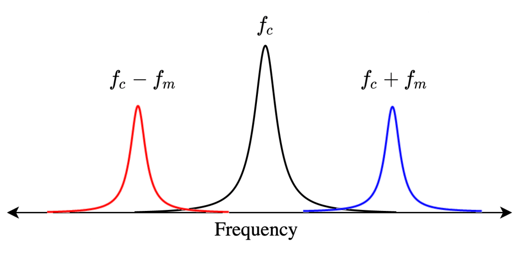
Let’s take a closer look at the circuit frequency measurement. As the vibrations of the drums modulate the LC circuit frequency, this shows up in frequency space as sidebands, two peaks which are separated from the circuit frequency $f_c$ by exactly the mechanical frequency $f_m$ of the oscillators (see image above). We call the peak at $(f_c - f_m)$ the red sideband, and the peak at $(f_c + f_m)$ the blue sideband. By sending a sequence of microwave pulses at these sideband frequencies, the authors are able to initialize, entangle, and readout the motional states of the two drums.

To see how this works, let’s focus on a single drumhead $\hat{b}$ coupled to an LC circuit $\hat{a}$ . If a red sideband pulse is applied, the interaction Hamiltonian is given by

$\hbar g(\hat{a}^{\dagger}\hat{b} + \hat{a}\hat{b}^{\dagger})$ .

(See derivation here. It’s straightforward but too long for this article.)

This acts like a phonon-photon swap operation, where a phonon of energy in the drum is converted into a photon of energy in the LC circuit at rate $g$ and vice versa. For example, when applied to the state $|1_m, 0_c \rangle$ (1 phonon, 0 photons), for a time $t = \pi/2g$ , the resulting evolution gives $|0_m, 1_c\rangle$ . If a blue sideband pulse is applied, the interaction is very different :

$\hbar g(\hat{a}^{\dagger}\hat{b}^{\dagger} + \hat{a}\hat{b})$

(See derivation here. It’s straightforward but too long for this article.)

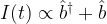
This interaction serves to generate an entangled photon-phonon pair. For example, when applied to the state $|0_m, 0_c \rangle$ , the resulting state takes the form (no normalization for simplicity) $|0_m, 0_c\rangle + \sqrt{p} |1_m, 1_c \rangle + \mathcal{O}(p)$ , where $p$ is the probability of generating an entangled pair.

Experimental Sequence

The experimental sequence in this work is in three steps: state preparation, where the drums are actively cooled to their motional ground state, entanglement, in which the motional state of the drums are entangled, and readout, in which the position and momentum fluctuations of the drums are measured. This sequence is repeated a large number of times, and the study looks at the correlations between $x_1$ , $x_2$ , $p_1$ , and $p_2$ .

State Preparation

Recall that at 10mK, the ~10MHz drums have an average of $n_m \approx 20$ phonons of vibrational energy. The drums should ideally be in their motional ground state $(n_m = 0)$ to maximize the fidelity of the entanglement protocol. A red sideband pulse can be used to cool the drums to their quantum ground state. Due to the swap interaction described above, a phonon of energy in the drum is converted into a photon of energy in the LC circuit. If the decay rate of the circuit is fast enough (which it is in this experiment), the converted photon is emitted out of the circuit before it can be swapped back into the drum. If the pulse is applied for a long enough time, phonons are continually removed from the drum until there are nearly 0. This ground-state cooling technique was first demonstrated in macroscopic objects 10 years ago, using microwave radiation and even optical radiation, and has worked remarkably well since.

Entanglement

To perform entanglement, the authors implement two pulses in parallel: a blue sideband pulse on drum 1, and a red sideband pulse on drum 2. The blue sideband pulse entangles a phonon in drum 1 and a photon in the LC circuit, then the red sideband converts the photon into a phonon in drum 2. The net effect is to generate a phonon in each of drum 1 and drum 2 which are entangled.

Readout

A blue sideband pulse can be used to measure the position and momentum of the drums (a red sideband pulse can be used for this too, but this work uses a blue sideband scheme). By sending a blue sideband pulse and looking at the reflected signal, the position and momentum of the oscillator can be indirectly probed.

It can be shown that the position and momentum of the drums are imprinted in the two quadratures of the reflected signal. For those unfamiliar, the quadratures of an oscillating signal $s(t)$ refer to the cosine and sine components of the signal:

$s(t) = I(t) \cos(\omega t) + Q(t)\sin(\omega t)$

$I(t)$ represents one quadrature, $Q(t)$ represents the other. In a blue sideband measurement, $I(t) \propto \hat{b}^\dagger + \hat{b}$ is proportional to position fluctuations and $Q(t) \propto \hat{b}^\dagger - \hat{b}$ is proportional to momentum fluctuations. The authors send in a blue sideband pulse and look at the reflected I and Q signals to extract the position and momentum of each drum. These I and Q measurements can be done relatively easily using standard microwave electronics.

Pulse sequence for entangling drums 1 and 2. Red indicates a red sideband pulse at frequency $f_c - f_m$ , whereas blue indicates a blue sideband pulse at frequency $f_c + f_m$ .

The full pulse sequence is shown above: this implements ground state preparation, entanglement, and readout of the two-drum mechanical state. The authors perform this pulse sequence a large number of times and record the values of ${x_1, x_2, p_1, p_2}$ , and plot the results. To show how the position and momentum of the drums are correlated, the authors plot each data point in phase space where the $(x, y)$ axes represent different combinations of ${x_1, x_2, p_1, p_2}$ . The authors do this for two different cases: no entangling pulse, and with entangling pulse, and examine the differences with each case.

Results

Position/momentum data for the ground state with no entangling pulse applied.

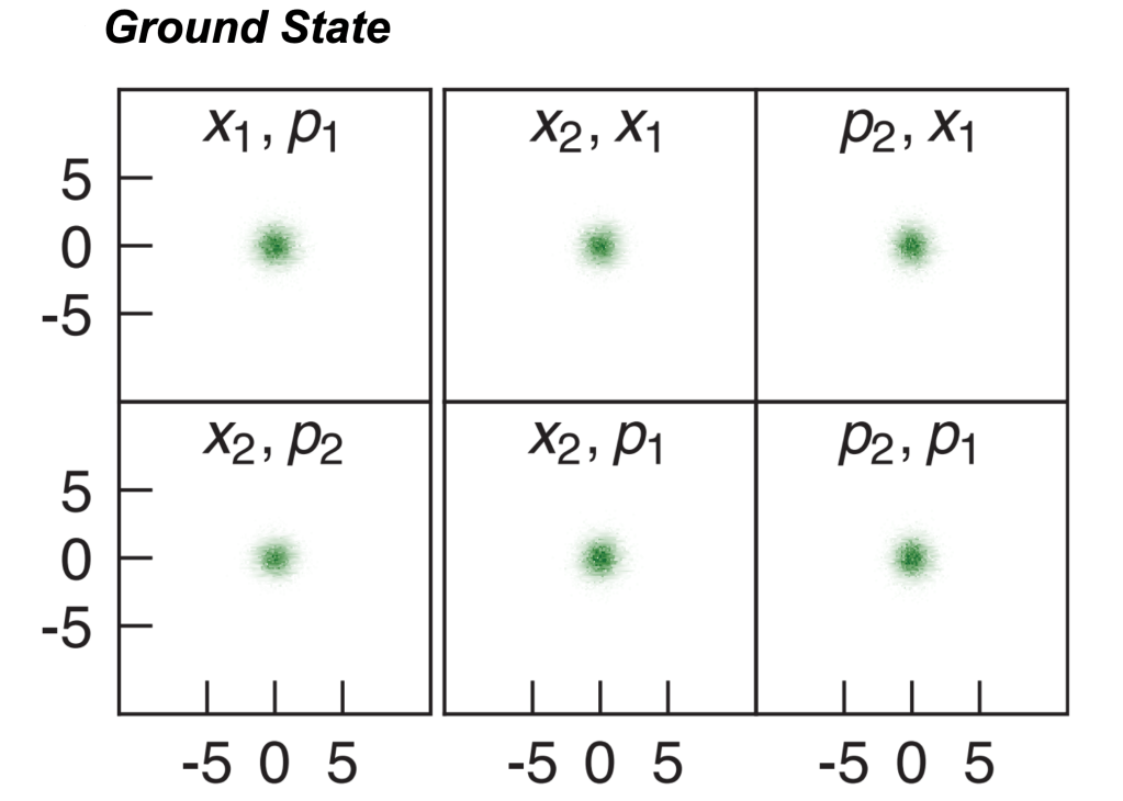
As expected, the position and momentum of the two drums showed no significant correlations for the data with no entangling pulse. The circular shape of the data in phase space indicates the fluctuations are randomly distributed and uncorrelated. From the magnitude of the fluctuations, the authors can also extract the average energy of the drums at $n_{m, 1} = 0.79$ and $n_{m,2} = 0.6$ phonons respectively, which indicates that the ground-state cooling is pretty successful.

Position/momentum data after an entangling pulse is applied.

The entangling pulse data tells a different story. The positions $x_1$ and $x_2$ are clearly correlated, while momenta $p_1$ and $p_2$ are clearly anti-correlated. This is a remarkable result as the two drums are physically separated and yet are moving in a coordinated way.

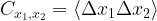
While the position/momentum data is impressive, these correlations could still be classical in nature. To verify that the correlated motion is a result of entanglement, the authors use the covariance matrix $C_{ij}$ , with elements defined by

$C_{ij} = \langle \Delta s_i \Delta s_j \rangle = \langle(s_i - \langle s_i \rangle)(s_j - \langle s_j\rangle)\rangle$

where $s_i$ can represent $x_1$ , $p_1$ , $x_2$ or $p_2$ . For example, $C_{x_1, x_2} = \langle \Delta x_1 \Delta x_2 \rangle$ . If two variables, say $x_1$ and $x_2$ are not correlated with one another, then $C_{x_1, x_2} = 0$ . If they are correlated, then $C_{x_1, x_2}$ will have some nonzero value.

According to the Simon-Duan criterion for entanglement, if the smallest eigenvalue $\nu$ of the partial transpose of the covariance matrix satisfies $\nu < 1/2$ , then the two-drum mechanical state is entangled. Covariance matrices for the two cases are shown below:

Covariance matrix for position/momentum data of the ground state and entangled state.

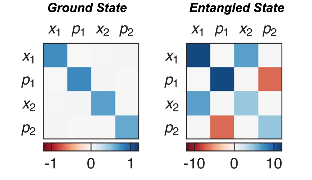
In the case with no entangling pulse, the position/momentum measurements for drums 1 and 2 were not correlated. Therefore the off-diagonal elements are nearly zero, and the covariance matrix is purely diagonal. After applying the entangling pulse, the covariance matrix looks quite different. The correlated nature of $x_1/x_2$ and $p_1/p_2$ creates off-diagonal elements in the covariance matrix. The authors find that by varying the entangling pulse time, the value of $\nu$ decreases below $1/2$ , verifying quantum entanglement for long enough entangling pulses. At the longest entangling time measured, $\nu$ is an order of magnitude below the entanglement threshold.

Pesky Pesky Noise

What makes observing quantum properties in macroscopic objects so difficult in the first place is the presence of environmental noise which corrupts the state of a macroscopic object. Ideally, one would like the measurements ${x_1, x_2, p_1, p_2}$ to reflect only position/momentum fluctuations, without any additional unwanted fluctuations. In practice, however, the I and Q measurements also contain vacuum noise, so that the position/momentum measurements take the form

$x_i = \sqrt{\eta_i}X_i + \sqrt{1 - \eta_i}\xi_i$ ,

$p_i = \sqrt{\eta_i}P_i + \sqrt{1 - \eta_i}\xi_i$

where $X_i$ , $P_i$ are the true values of position/momentum, $\xi_i$ is the vacuum noise of each I/Q measurement (basically just a random variable with variance 1/2), and $\eta_i$ is the measurement efficiency. If the value of $\eta$ is small enough, then the measurements of ${x_1, x_2, p_1, p_2}$ become corrupted with noise, and true entanglement becomes hard to verify. The measured value of $\nu$ differs from the true value by

$\nu_{\mathrm{meas}} = \eta \nu + (1 - \eta)\cdot 1/2$

where $\eta = \sqrt{\eta_1\eta_2}$ is the geometric mean of the efficiencies. The smaller the value of $\eta$ , the closer $\nu_{\mathrm{meas}}$ is to $1/2$ and the harder it is to verify the $\nu<1/2$ threshold. The authors show the calculated value of $\nu$ as a function of entangling pulse time:

Measured values of $\nu$ (left) and extracted true values of $\nu$ (right) vs. entangling pulse duration. $\nu < 0.5$ indicates the threshold for quantum entanglement.

Measured values of $\nu$ (left) and extracted true values of $\nu$ (right) vs. entangling pulse duration. $\nu < 0.5$ indicates the threshold for quantum entanglement.

The authors find that even without calibrating out the noise in their measurements, they obtain values of $\nu_{\mathrm{meas}}$ that are >40% below the entanglement threshold for the longest pulse time in this work. This is a remarkable result: the authors are able to observe macroscopic entanglement directly from the measured data, even in the presence of noise!

To summarize, this work demonstrates the ground-state cooling, entanglement, and measurement of the quantum motional states of two mechanical oscillators. The authors observe quantum behavior of the collective motion of billions of atoms, further confirming that even large objects can be described with a quantum-mechanical wavefunction. The results of this work pave the way for many unanswered questions: how large can a system get and still behave quantum-mechanically? Will gravity destroy quantum states at some intermediate size? Can we use entanglement in large objects as a resource for quantum computing? This work is an exciting step in the long road ahead towards answering these questions.