Just How Much Better is Quantum Machine Learning than its Classical Counterpart?

Title: Information-theoretic bounds on quantum advantage in machine learning

Authors: Hsin-Yuan Huang, Richard Kueng, John Preskill

First Author’s Institution: California Institute of Technology

Status: Pre-print on arXiv

In the past few years, machine learning has proven to be an extremely useful computational tool in a variety of disciplines. Examples include natural language processing, image recognition, beating players at Go, quantum error correction, and shifting through massive quantities of data at CERN. As is often the case, we may choose to ponder whether replacing classical algorithms by their quantum counterparts will yield computational advantages.

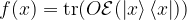
The authors consider the complexity of training classical machine learning (CML) and quantum machine learning (QML) algorithms on the class of problems that map a classical input (bit string) to a real number output through any physical process (including quantum processes). The goal of the ML algorithms is to learn functions of the following form: $f(x) = \text{tr}(O \mathcal{E}(\left|x\right>\left<x\right|))$ . Unpacking the notation, we see that given some input bit string $x\in \{0,1\}^n$ that designates an initial quantum pure state, we get an output by processing the input through a quantum channel $\mathcal{E}$ and then determining the expectation value of an operator $O$ with respect to the output of the channel (i.e. quantum evolution of the initial state). The ML algorithms will attempt to predict the expectation value of $O$ after training on many input bit strings and channel uses. You may wonder whether a single bit string is a sufficiently complicated input, but recall that all of the movies you watch, the articles on Wikipedia you read, and the music you play on your computer are represented by bit strings. Given a sufficiently long input bit string, we can feed into our algorithm arbitrarily long and precise classical data. What is very interesting about this class of problems is that we can describe quantum experiments with many different input parameters in this language, meaning the ML algorithms are being trained to predict the outcome of (potentially very complicated) quantum physical experiments. This could include predicting the outcome of quantum chemistry experiments, determining the ground state energy of a system, or predicting a variety of other observables from a myriad of physical processes.

As is often the case, there isn’t a single clear answer to the question posed, but the authors discuss two scenarios of interest. First, a secnario in which QML models pose no significant advantage over CML models and another in which QML models provide exponential speedup. According to the paper, if one consider’s minimizing average prediction error (over a distribution of all the inputs), then QML does not provide a significant advantage over classical machine learning. However, if one is interested in minimizing worst-case prediction error (on the single input with the worst error), then quantum machine learning requires exponentially fewer runs of the quantum channel.

What are the ML Models of Interest?

The goal of supervised machine learning is to use a large quantity of input data and a corresponding set of outputs to train a machine to generate accurate predictions from new data. In this paper, the objective is to see how many times it is necessary to run a physical process $\mathcal{E}$ such that the machine can accurately predict the results of the experiments to some tolerance. The scaling of the number of times the quantum process $\mathcal{E}$ is used in the training phase of the algorithm defines the complexity of the algorithm. Each of the ML algorithms generates a predictive function $h(x)$ , where the prediction error on each input is given by $\left|h(x_i)-f(x_i)\right|^2$ . If given a probability distribution $\mathcal{D}(x)$ over all possible inputs, we would like to figure out the number of times that $\mathcal{E}$ must be run to either produce an average-case prediction error of $\sum_{x\in\{0,1\}^n} \mathcal{D}(x)\left|h(x)-\text{tr}(O\mathcal{E}(\left|x\right>\left<x\right|))\right|^2 \leq \epsilon$ or a worst-case prediction error given by $\text{max}_{x_i\in\{0,1\}^n}\left|h(x_i)-f(x_i)\right|^2\leq \epsilon$ .

The quantum advantage arises only when one considers the worst-case prediction error instead of the average prediction error.

It is very reasonable to think quantum machine learning would be better than classical machine learning when trying to predict the outputs of quantum experiments, but the main result throws that assumption into question. We begin by explaining how QML and CML are defined.

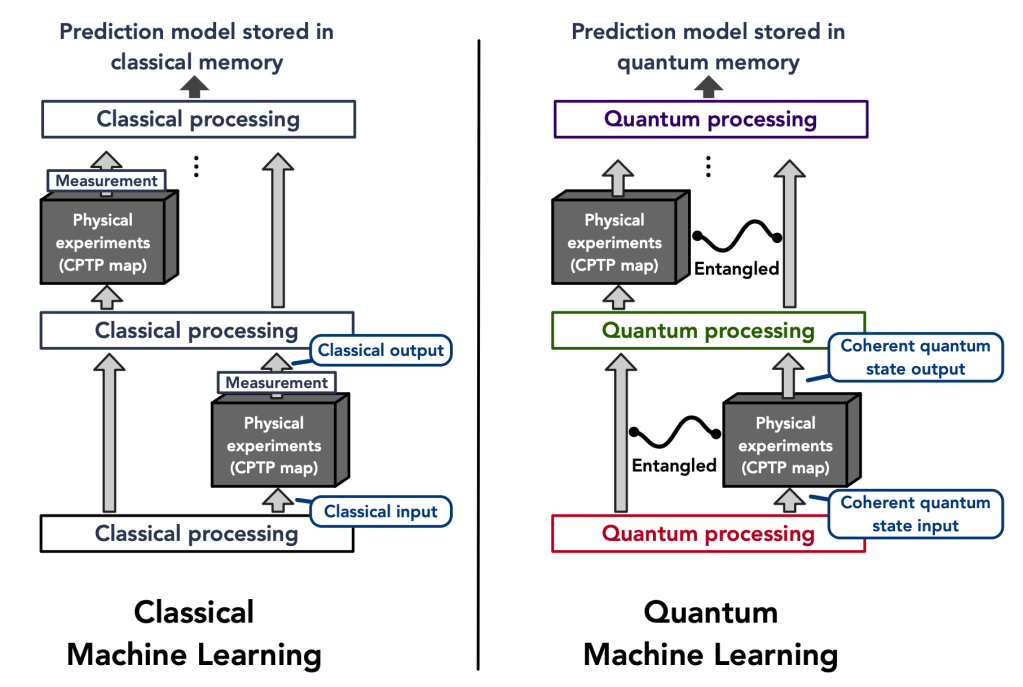
Figure 1: Illustration of classical and quantum machine learning models (Figure 1 from article)

Classical ML models are composed of a training phase that consists of taking a randomized set of inputs $x_i$ and performing quantum experiments defined by a physical map (a CPTP map) from a Hilbert space of $n$ qubits to one of $m$ qubits that yields an output quantum state for each input. However, CML needs to be trained on classical output and so a POVM measurement (which is a generalization of a projective measurement) is performed that yields an output $o_i \in \mathbb{R}$ . Any classical machine learning algorithm (neural networks, kernel methods, etc.) can then be applied to generate the predictive function $h(x)$ that approximates $f(x)$ (the true function) from the set of pairs of inputs and classic outputs $\{(x_i,o_i)\}_{i=1}^{N_c}$ . Here $N_c$ denotes the number of times that applying the channel $\mathcal{E}$ is required for CML since it is only possible to obtain one input/output pair per channel usage. The authors present a further restricted classical ML algorithm, which is identical to the general case, but where instead of doing arbitrary measurements to generate the outputs, only the target observable $O$ is directly measured.

A quantum ML model has the same goal as the classical models, but has the added advantage that the algorithm can be trained directly on quantum data. The general flow is that given an initial state $\rho_0$ on many qubits, the quantum channel $\mathcal{E}\otimes \mathbb{I}$ is applied $N_Q$ times with quantum processing maps $\mathcal{C}_i$ inserted in between $\mathcal{E}$ applications. The quantum data processing maps take the place of the classical machine learning algorithms. The resultant state that is stored in quantum memory is the learned prediction model. To predict new results, the final state after all of the channel applications and processing ( $\rho_{Q}$ ) is measured differently based on the desired input bit strings $\tilde{x}_i$ . The outcomes of these measurements are the outputs of the predictive function $h_Q(\tilde{x}_i)$ that approximate the desired function $f(\tilde{x})$ .

The Meat of the Paper

Average-case Prediction Error Result

The main results of the paper are presented in the form of theorems. The first theorem shows that if there exists a QML algorithm with an average prediction error bounded by $\epsilon$ that requires $N_Q$ uses of the channel $\mathcal{E}$ , then there exists a restricted CML algorithm with order $\mathcal{O(\epsilon)}$ average prediction error that requires $\mathcal{O}\left(\frac{m N_q}{\epsilon}\right)$ channel uses. The training complexity of the classical algorithm is directly proportional to that of the quantum model up to a factor of $\frac{m}{\epsilon}$ where $m$ is the number of qubits at the output of the map $\mathcal{E}$ .

Sketch of First Theorem Proof

Consider an entire family of maps $\mathcal{F}$ that contains the map $\mathcal{E}$ of interest. Cover the space of the family of maps with a net by choosing the largest subset of maps $\mathcal{S}=\{\mathcal{E}_a \}_{a=1}^{|\mathcal{S}|} \subset \mathcal{F}$ such that the functions generated by different maps $f_a(x) = \text{tr}\left(\mathcal{O} \mathcal{E}_a (\left|x\right>\left<x\right|)\right)$ are sufficiently distinguishable over the distribution of inputs $\mathcal{D}(x)$ . (In the paper they take the average-case error between any two different elements of $\mathcal{S}$ to be at least $4\epsilon$ ).

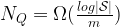
The proof proceeds as a communication protocol that starts by having Alice choose a random element of the packing net ( $\mathcal{E}_a \in \mathcal{S}$ ). Alice then prepares the final quantum state $\rho_{\mathcal{E}_a}$ by using the chosen channel $N_Q$ times and interleaving those uses with the quantum data processing maps $\mathcal{C}_i$ . This results in the state the QML algorithm is supposed to generate to make predictions through measurements. Alice then sends $\rho_{\mathcal{E}_a}$ to Bob and hopes he can determine what element of the packing net she initially chose by using the predictions of the QML model. Bob can then generate the function $h_{Q, a}(x)$ that approximates $f_{a}(x)$ with low average-case prediction error by construction. Moreover, because the different elements of the packing net are guaranteed to be far enough apart, Bob can with high-probability determine which element Alice chose. Assuming Bob could perfectly decode which element Alice sent, Alice could transmit $log|\mathcal{S}|$ bits to Bob. With this scheme we expect the mutual information (a measure of the amount of information that one variable can tell you about another) between Alice’s selection and Bob’s decoding to be on the order of $\Omega(log|\mathcal{S}|)$ bits. The authors now make use of Holevo’s theorem, which provides an upper bound on the amount of information Bob is able to obtain about Alice’s selection by doing measurements on the state $\rho_{\mathcal{E}_a}$ . This is on the order of the previously given mutual information, however, it is also possible to relate the Holevo quantity directly to the number of channel uses $N_Q$ required to prepare the state Bob receives. Through an induction argument in the Appendix, the authors show the Holevo information is upper bounded by $\mathcal{O} (m N_Q)$ . From this it follows that the number of channel uses for the quantum ML algorithm is lower-bounded by $N_Q = \Omega( \frac{log |\mathcal{S}|}{m})$ .

All that’s left is to relate the number of channel uses required for the QML model to the necessary number needed for the classical machine learning algorithm. A restricted CML is constructed such that random elements $x_i$ are sampled from $\mathcal{D}(x)$ and the desired observable is measured after preparing $\mathcal{E}(\left|x_i\right>\left<x_i\right|)$ each time. As mentioned earlier, $N_c$ experiments are performed. The pairs of data $\{(x_i,o_i)\}^{N_c}$ are used to perform a least-squares fit to the different functions $f_a(x)$ of the packing net, which are sufficiently distinguishable as defined earlier. Therefore, given a sufficiently large number of data points, it is possible to determine which element of the packing net was used as the physical map from the larger family of maps. The authors show that if the number of points obtained $N_c$ is on the order of $\mathcal{O}\left(\frac{log|S|}{\epsilon}\right)$ , it is possible to find a function that achieves an average-case prediction error on the order of $\epsilon$ . Relating $N_c$ and $N_Q$ through $log|\mathcal{S}|$ directly yields that $N_c = \mathcal{O}\left(\frac{m N_Q}{\epsilon}\right)$ . Hence, if there is a QML model that can approximately learn $f(x)$ , then there is also a restricted CML model that can approximately learn $f(x)$ with a similar number of channel uses. This means that there is no quantum advantage in terms of the training complexity when considering minimum average-case prediction error as any QML model could be replaced by a restricted CML model that achieves comparable results.

Worst-case Prediction Error Result

The second main result states that if we instead consider worst-case prediction error, then an exponential separation appears between the number of channel uses necessary in the QML and CML cases. This is shown in the paper through the example of trying to predict the expectation values of different Pauli operators for an unknown $n$ -qubit state. As a refresher, the Pauli operators ( $I, X, Y, \text{and } Z$ ) are 2×2 unitary matrices that form a basis for Hermitian operators, which correspond to observable operators in quantum mechanics. Since any Hermitian operator can be decomposed in terms of sums of Paulis, it is natural to wonder about the different expectation values of each Pauli operator given an unknown state. Given a $2n$ -input bit string we can specify an $n$ -qubit Pauli operator $P_x$ and the channel $\mathcal{E}$ , which both generates the unknown state of interest and maps $P_x$ to a fixed observable $O$ . Therefore, the function we are getting the ML model to learn is $f(x) = \text{tr}\left(\mathcal{O} \mathcal{E}_{\rho} (\left|x\right>\left<x\right|)\right) = \text{tr}\left(P_x \rho\right)$ . The authors show that by cleverly breaking the QML model into two stages, the first of which is estimating the magnitude of the expectation value ( $|\text{tr}(P_x \rho)|$ ) and the second estimating the sign of the expectation value, only $N_Q = \mathcal{O}\left(\frac{log(M)}{\epsilon^4}\right)$ channel uses are necessary to predict expectation values of any $M$ Pauli observables. Therefore it is possible to predict all $4^n$ Pauli expectation values up to a constant error with only a linear scaling in the number of qubits ( $\Omega(n)$ ). On the other hand, the paper shows the lower bound for estimating all the expectation values of the Pauli observables using classical machine learning is $2^\Omega(n)$ . Therefore, there is an exponential separation between QML and CML models in the number of channel uses necessary for predicting all Pauli observables in the worst-case prediction error scenario. The authors numerically demonstrate the difference in complexity between the different types of algorithms and show the separation clearly exists for a class of mixed states, but vanishes for a class of product states.

Takeaways

Classical machine learning is much more powerful than may be naively assumed. For average-case prediction error, CML models are capable of achieving a comparable training complexity to QML models. This means we may not need not to wait for QML to predict the outcomes of physical experiments. Performing quantum experiments and using the output measurements to train CML models is a process that can be implemented in the near-term. In the case of approximately learning functions it appears that using a fully quantum model does not provide a significant advantage. However, the authors did demonstrate an interesting class of problems in which QML models are capable of exponentially outperforming even the best possible classical algorithm. The question is whether there are interesting tasks that require having a minimum worst-case prediction error, where learning the function over a majority of inputs does not suffice. I leave it to the reader as an exercise to search out other interesting learning tasks where quantum advantage is achieved and where the classical world of computing does not suffice.

Ariel Shlosberg is a PhD student in Physics at the University of Colorado/JILA. Ariel’s research focuses on quantum error correction and finding quantum communication bounds and protocols.