What can quantum information tell us about the foundations of statistical mechanics?

By Mauro E.S. Morales

Title: Entanglement and the foundations of statistical mechanics

Authors: Sandu Popescu^1,2, Anthony J. Short¹, Andreas Winter³.

Institutions: ¹H. H. Wills Physics Laboratory, University of Bristol, Tyndall Avenue, Bristol BS8 1TL, UK

²Hewlett-Packard Laboratories, Stoke Gifford, Bristol BS12 6QZ, UK

³Department of Mathematics, University of Bristol, University Walk, Bristol BS8 1TW, UK

Manuscript: Published in Nature [1], Open Access on arXiv [2]

It is sometimes easy to forget, that in addition to the impact it has had on the development of new technologies, the ongoing development of quantum information theory has had implications on the foundations of Physics itself. In fact, based on insights from quantum information, in [1] the authors argue for re-framing a fundamental principle that lies is at the very basis of statistical mechanics, namely the equal probability postulate.

The concept of a thermodynamic “equilibrium” is central to classical statistical mechanics. In such an equilibrium, one can assume that there are no macroscopic changes in a given system. Consider a box full of solid particles inside, and take this box to be connected to a heat bath of temperature $T$ and isolated from everything else. For a given temperature, we know that the probability that the system is in a state with energy $E_i$ is given by

$P(E_i)=\frac{1}{Z}e^{-E_i /kT} ,$

where $Z$ is the well-known partition function, which roughly tells us how many different ways one can partition a system into subsystems having the same energy, and $k$ is the Boltzmann constant which relates absolute temperature to the kinetic energy of each microscopic particle in any given system.

A key assumption in this is that all possible states of the “total system”, which encapsulates the box and the bath, have equal probability. This assignment of probabilities to each energy is known as the canonical ensemble. Physicists also work with other types of ensembles, for instance, the micro-canonical ensemble, where the total energy is fixed and all states have equal probability. It is important to stress that this is an assumption on the total system, not something that is proven from other postulates. In other words, we postulate this a priori.

A general canonical principle

In [1], the authors propose a way to derive probabilities assigned by the canonical ensemble by explicitly considering quantum systems. In fact, their methods prove a more general canonical principle than the classical one, and we shall elaborate on this general principle further.

First, let us consider a large isolated quantum system $R$ described by a Hilbert space $\mathcal{H}_R$ which is decomposed into a system $S$ with Hilbert space $\mathcal{H}_S$ and an environment $E$ with Hilbert space $\mathcal{H}_E$ . In principle $\mathcal{H}_R$ could be described by $\mathcal{H}_S\otimes \mathcal{H}_E$ , but we can consider restrictions over the space as shown in the picture below.

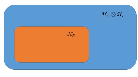
This restriction would make the space $R$ smaller and would be analogous to the system presented in the introduction with a fixed temperature $T$ . In a quantum setting, such restrictions are described by considering constraints on the possible joint states of system $S$ and $E$ . We note that such restrictions need not be related solely to temperature, it can in fact be any type of constraint whatsoever on the total system, a feature that will turn out to be important for the generality of the proof.

We can consider as in classical thermodynamics, the state that gives equal probability to all states in $\mathcal{H}_R$ , which can be represented using the identity matrix. This state gives equal probability to all states of $R$ , assuming that $R$ is in this state is akin to the assumption in the combined box/bath example in the introduction.

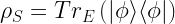
In this case, the canonical state would be obtained by tracing out the degrees of freedom from the bath. We denote this state as $\Omega_S$ . If we had taken the system $R$ as the box/bath combined with the restriction of the temperature $T$ , then $\Omega_S$ would correspond to the Gibbs state, which describes an equilibrium probability distribution that remains invariant under any future evolution of the system, with the probabilities given in the introduction. So far, we have just rewritten everything in the language of quantum mechanics but the authors take a step further. It’s important to remark that we could have taken any other restriction for $\mathcal{H}_R$ and the canonical state would be different from the canonical thermal canonical state defined earlier in the introduction.

What if the state of $R$ is not the identity?

If the state of $R$ corresponds instead to some state $|\phi\rangle \langle \phi |$ and defines the state of the system $S$ as $\rho_S=Tr_{E}\left( |\phi\rangle \langle \phi |\right)$ , then the authors show that $\rho_S$ is close to the state $\Omega_S$ for almost all possible states $|\phi\rangle \langle \phi |$ . This implies that there is no need to assume equal probability for all states since, as we will see, most of the states in system $R$ will give the correct canonical state in $S$ .

In quantum information, we can measure how close two states are from each other using the so-called trace distance. We will denote the distance between $\rho_S$ and $\Omega_S$ as $D(\rho_S,\Omega_S)$ .

This distance represents the maximal difference between the two states in the difference of obtaining any measurement. In other words, the trace distance tells us how hard is to tell apart $\rho_S$ and $\Omega_S$ apart under measurements (the greater the distance, the harder to tell apart).

Distance between density matrices is defined by D

To understand what the authors prove let’s set some notation. Let $\rho_S (\phi)=Tr_{E}\left( |\phi\rangle \langle \phi |\right)$ be the state obtained by tracing out the environment and define the set of states at a distance of the canonical state equal or greater to $\eta$ as $\mathcal{S}$ . The radius defined by $\eta$ is shown below.

Note that $\mathcal{S}$ is a set in the Hilbert space $\mathcal{H}_R$ (different from the one pictured above, which is the space of density matrices). We picture below the set $\mathcal{S}$

The set $\mathcal{S}$ fills a volume in the Hilbert space, we denote the fraction of states at distance equal or greater to $\eta$ of the canonical state as

$\frac{V\left(\mathcal{S}\right)}{V\left(\mathcal{H}_R\right)}$

where $V(\cdot)$ refers to the “volume” of the set in the argument. Another way of interpreting this ration is as the probability of picking a random state $|\phi\rangle$ such that the distance of $\rho_S$ to the canonical state is equal or greater to $\eta$ .

What the authors prove rigorously is that this probability gets smaller (in fact exponentially smaller) as $\eta$ grows. More precisely they prove that for $\epsilon>0$ we have that

$\frac{V\left(\mathcal{S}\right)}{V\left(\mathcal{H}_R\right)}\leq \eta'$

with $\eta\approx\epsilon$ and $\eta'=4 \exp(-Cd_R \epsilon^2)$ .

Note that as $\epsilon$ grows, the probability, of picking a state such that the distance is big enough, decays exponentially.

We won’t go into the full intricacies of the proof for this statement, but we will mention that a key ingredient is Levy’s lemma (for those curious about this Lemma, see [2]). This lemma has in fact seen use in other areas of quantum information. Those familiar with variational quantum algorithms may have heard of barren plateaus, which limit the trainability of variational circuits [3]. Levy’s lemma is a key ingredient in proving that under certain conditions barren plateaus become inevitable when training these quantum circuits.

References

[1] Popescu, S., Short, A. & Winter, A. Entanglement and the foundations of statistical mechanics. Nature Phys 2, 754–758 (2006). https://doi.org/10.1038/nphys444

[2] Popescu, S., Short, A. & Winter, A. The foundations of statistical mechanics from entanglement: Individual states vs. averages. arXiv:0511225 [quant-ph], Oct. 2006.

[3] McClean, J.R., Boixo, S., Smelyanskiy, V.N. et al. Barren plateaus in quantum neural network training landscapes. Nat Commun 9, 4812 (2018). https://doi.org/10.1038/s41467-018-07090-4

A general canonical principle

What if the state of is not the identity?

Share this:

Like this:

Leave a Reply Cancel reply

What if the state of $R$ is not the identity?