This post was sponsored by Tabor Electronics. To keep up to date with Tabor products and applications, join their community on LinkedIn and sign up for their newsletter.
Authors: Dhruv Devulapalli, Eddie Schoute, Aniruddha Bapat, Andrew M. Childs, Alexey V. Gorshkov
arXiv: https://arxiv.org/abs/2204.04185
Background and motivation
When we write quantum circuits on paper or in software, it’s often convenient to assume that any pair of qubits are connected. It’s convenient both (i) as a level of abstraction – we sometimes don’t want to think about low-level hardware details when thinking about algorithms – and (ii) because it’s in some sense true – even if there’s not a direct edge between two qubits, as long as there is some connected path the qubits can interact. This is exhibited in the figure below.
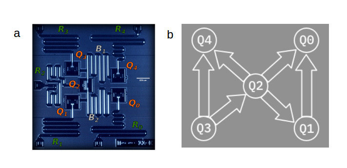
In the left panel, this figure shows a five-qubit superconducting processor from IBMQ, and highlights the qubit connections in the right panel. Qubit Q0 and Q1 are directly connected, but qubit Q0 and Q3 are not. However, there is a connected path from qubit Q0 to Q3, namely the path Q0 – Q2 – Q3. Because there is a connected path, two-qubit operations can be performed between qubits Q0 and Q3.
How is this possible? Swapping two qubits is a unitary operation – indeed a self-inverse operation – and so a permissible quantum operation. Furthermore, it’s safe to assume that this is a readily available operation on a quantum computer. Indeed, we can compose a swap operation out of three controlled-not (CNOT) operations, and CNOTs are commonly assumed to be a primitive operation on a quantum computer. A CNOT is defined as
where a and b are bits and ⊕ denotes addition modulo two. In words, the second qubit is flipped if the first qubit is in the |1⟩ (excited) state. The subscript “12” indicates that qubit 1 is the control and qubit 2 is the target. If we swap this indices, then
From this, a little algebra shows that the composition of three CNOTs implements a swap operation:
So, we can assume we have such a swap operation (SWAP) available between connected qubits.
In the above figure, qubits Q0 and Q3 weren’t directly connected, but they were both connected to qubit Q2. If we swap the state of Q0 and Q2, then there is now a direct connection between Q0 and Q3, and we can perform a two-qubit gate. If we’d like, after the two-qubit gate we can SWAP Q0 and Q2 again to restore the previous configuration. It’s easy to generalize this to any pair of qubits which have a connected path between them. Such a sequence of SWAPs is known as a SWAP network, and the general task of “getting qubits where they need to be” is known as qubit routing. The word “routing” is used in reference to packet switching on networks, for example the internet, a task with many common features.
Thus it’s safe to assume that we can perform a two-qubit gate between any pair of qubits. The downside is the additional SWAP operations needed to do so. Quantum computers are noisy and each operation has some probability of error, so the more operations there are the more likely it is for an error to occur. It is thus of great interest and practical importance to develop procedures to perform qubit routing with the fewest possible resources, i.e., with the shortest possible depth.
Main idea and results of the paper
This paper focuses on performing qubit routing with the fewest possible resources, and in particular considers a clever qubit routing procedure based on teleportation. These authors weren’t the first to consider teleportation for qubit routing, but they analyze it in novel ways. As we will discuss below, teleportation requires local operations (including measurements) and classical communication, abbreviated LOCC. As such, the author’s scheme can be referred to as LOCC routing in general and teleportation routing in particular. Here, we use “TELE routing” to mean teleportation-based routing and “SWAP routing” to mean SWAP-based routing.
The authors’ main strategy is to define metrics for how well qubit routing algorithms perform, then compare TELE routing to SWAP routing in three main categories. What are the three categories? A routing problem is defined by a quantum computer you want to run on and a circuit you want to run. More abstractly, we represent a quantum computer by a graph G where nodes (vertices) are qubits and edges are connections between qubits, and we represent a circuit as a permutation π of the graph. (We don’t care about the operations here, only how to route the qubits, so it’s sufficient to represent the circuit as a permutation.) So, a routing problem is defined by a graph G and a permutation π. The three categories the authors consider are:
- A specific graph G and a specific permutation π.
- A specific graph G and any permutation π.
- Any graph G and any permutation π.
The main results in each category, colloquially stated, are:
- There exists a graph G with N nodes and a permutation π such that SWAP routing takes depth of order N and TELE routing takes constant depth independent of N.
- There exists a graph G with N nodes such that, for any permutation π on G, SWAP routing takes depth log N and TELE routing takes constant depth independent of N.
- For any graph G with N nodes and any permutation π on G, the maximum advantage of TELE routing over SWAP routing is of order (N log N)½.
The remainder of this article is an invitation to understanding these results, starting with a review of teleportation then walking through the simpler results while providing intuition for the others.
Teleportation
Since we are going to use teleportation as a subroutine for qubit routing, let’s quickly (re-)analyze the protocol. The quantum circuit for teleportation is shown below.
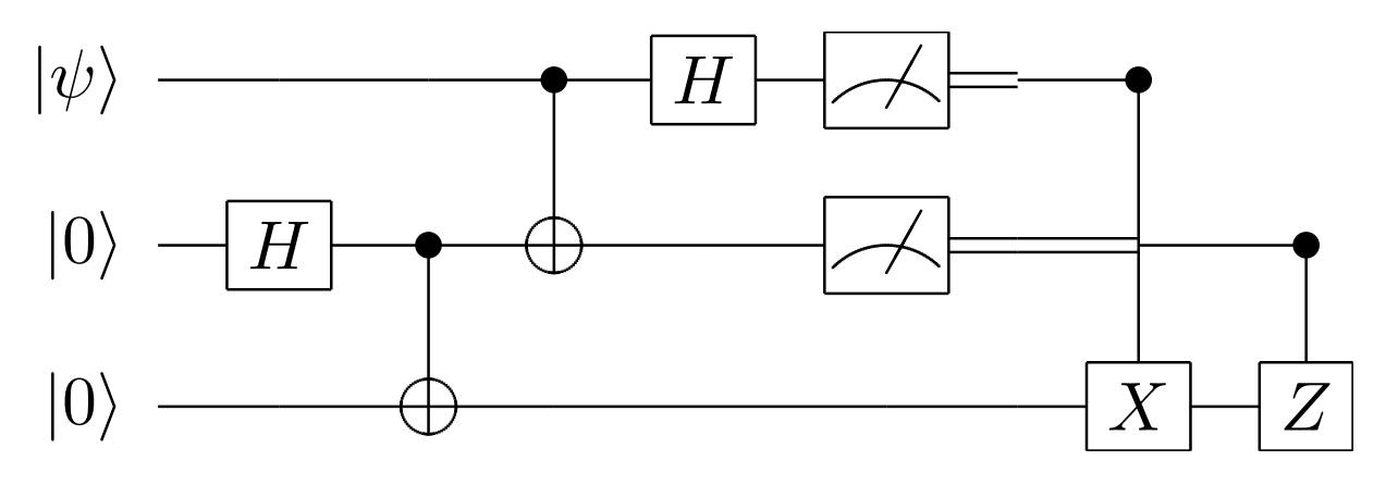
This circuit “teleports” an arbitrary quantum state |𝜓⟩ = α|0⟩ + β|1⟩ on the first qubit to the third qubit by means of local operations (both unitary operations and measurements) and classical communication. Concretely, “classical communication” means performing operations conditional on the measurement outcomes (classical information) of the first two qubits. Because sending this classical information cannot be instantaneous, the name “teleportation” is not to be taken in a literal sense.
We can understand the above circuit for teleportation as follows. The Hadamard and CNOT create a Bell state on the last two qubits. (We omit normalization here and throughout.)
After, we measure the top two qubits in the Bell basis, which corresponds to the Bell state preparation circuit in reverse. Before the measurements, one can show with a little algebra that the final state of the three qubits is as follows (again omitting normalization):

Written this way, it’s easy to see how to always obtain the state |𝜓⟩ on the third qubit after measuring the first two qubits:
- If we measure |00⟩ (the first term in the above equation), the state of the third qubit is |𝜓⟩
- If we measure |01⟩ (the first term in the above equation), the state of the third qubit is X|𝜓⟩. Perform X to obtain |𝜓⟩.
- If we measure |10⟩ (the first term in the above equation), the state of the third qubit is Z|𝜓⟩. Perform Z to obtain |𝜓⟩.
- If we measure |11⟩ (the first term in the above equation), the state of the third qubit is XZ|𝜓⟩. Perform XZ to obtain |𝜓⟩.
Thus we always obtain |𝜓⟩ on the third qubit. Now that we have one three-qubit “gadget” for teleportation, we can consider chaining several of these gadgets together to teleport a qubit a greater distance. This is illustrated in Figure 1 of the paper:
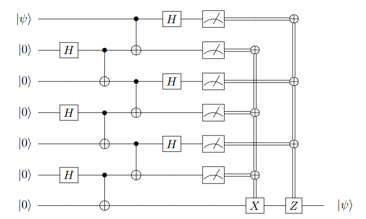
Notice the very nice property that the depth of this seven-qubit teleportation circuit is the same as the depth of the three-qubit teleportation circuit. Specifically, both circuits have a depth of four. This is different from using SWAP routing in which the SWAPs have to be sequential as shown below.

Here, the depth of the circuit grows with the number of qubits. This observation is key to understanding why and when teleportation-based routing may be advantageous.
Routing time, and bounds
Let rt(G, π) denote the routing time (minimum circuit depth) to perform the permutation π on the graph G. Let rt(G) denote the worst-case routing time taken over all permutations on G.
Note that any SWAP routing procedure can be “mimicked” by a TELE routing procedure which simply substitutes each SWAP operation with a teleportation gadget, using the same (constant) depth. But, it’s possible for TELE routing to be faster. Therefore, the time for TELE routing is at most the time for SWAP routing.
In prior work, it has been shown that SWAP routing on a graph G with N nodes takes O(N) time. Combining this with the previous argument, we also have that TELE routing takes O(N) time.
In summary, so far we have TELE routing time ≤ SWAP routing time = O(N) on a graph G with N nodes.
It’s also possible to show lower bounds. Since swapping two nodes at a distance d requires at least d SWAPs, we have that the SWAP routing time is at least diam(G). (The diameter of a graph G is the maximum shortest-path distance between any pair of nodes.) This is referred to as the “diameter lower bound” in the paper.
The diameter bound doesn’t apply to TELE routing, but it is possible to provide a lower bound for this. Leaving the proof to an unpublished article by the same authors, the authors provide the bound

where c(G) is the vertex expansion of G and, for connected graphs, is between 2 / N and 1. LOCC routing is the most general, so this implies SWAP routing ≥ TELE routing ≥ 2 / c(G) – 1.
TELE routing vs SWAP routing
Define the teleportation advantage adv(G, π) as the ratio of SWAP routing to TELE routing, i.e.

Category 1: A specific graph G and a specific permutation π
The first case the authors consider is shown below.

Here we have G as a line graph (hollow black nodes with black lines as edges) and π as the permutation which swaps the left-most and right-most qubits. If there are N nodes in G, SWAP routing takes depth of order N because each SWAP must be in parallel. However, as we have seen above, the depth of TELE routing is constant in N. Therefore the teleportation advantage adv(G, π) is of order N, a significant advantage!
The second case the authors consider is similar, shown below.

Here we have the same graph G but a “rainbow permutation” π, so-called because the red lines form a rainbow as drawn above. The parameter 0 < α < 1 quantifies how many nodes appear in the rainbow permutation. By the diameter bound, SWAP routing as depth N. For TELE routing, one can swap each pair of nodes sequentially with a constant depth circuit. Since there are Nα / 2 pairs of nodes in the permutation, TELE routing takes depth Nα / 2. So, the teleportation advantage in this case is O(N1 – α). This is sublinear for nonzero α, so less than the linear advantage for the first case, but still advantageous.
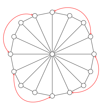
One might suppose TELE routing is only advantageous because the diameter of the line graph in the above examples was of order N (the number of nodes). But now consider wrapping the line graph around so two end nodes are connected in a circle. Further, place an additional node in the center of the circle with an edge to every node on the circumference, as shown below.

The diameter of this graph, the so-called “wheel graph” or WN, is constant, independent of the number of nodes N. (Specifically, the diameter is two.) Now consider the permutation shown in red on this graph. This permutation swaps qubits at a distance l along the “rim” of the wheel. As the authors argue, the SWAP routing time for this case is min(3l, N / l – 1). The 3l corresponds to using the central node to SWAP every pair of qubits sequentially, and the N / l – 1 corresponds to swapping qubits along the rim of the wheel in parallel. Now, for TELE routing, this permutation on G can be done in constant depth by simply teleporting each pair of qubits along the rim in parallel. If we set l to be the square root of N / 2, this yields the maximum teleportation advantage of

Thus, teleportation routing enables super-diametric speedups.
Category 2: A specific graph G and any permutation π
In the above example we got to hand-pick the permutation π. Now let’s consider the more general case of any permutation π, and ask if we can find some graph G where TELE routing is advantageous.
The authors show the answer to this question turns out to be yes: there exists a graph G with N nodes where SWAP routing takes depth at least logarithmic in N, and TELE routing takes constant depth independent of N. The graph G which achieves this is shown below.

This graph has n layers of subgraphs vertically stacked on top of each other. As such, the authors call it L(n). The nth layer is a complete graph on 2n nodes, shown with blue edges above. These layers are stacked by connecting every node in the current layer to the layer below it, shown with black edges above. For example, the first layer K1 has one node, and an edge to each node in the layer K2 below. The layer K2 has two nodes, and each node is connected to every node in the layer K4 below it. And so on. The total number of nodes in L(n) is 2n – 1. Imagine building a quantum computer with this topology!
The proofs of the SWAP routing and TELE routing depths quoted above are somewhat involved, so we omit them here and refer the interested reader to the paper (see Sec. V).
Category 3: Any graph G and any permutation π
Last, the authors consider the most general category of any graph G and any permutation π. For this case, the relevant metric is the “maximum teleportation advantage”

The authors prove (Theorem 6.4) that

Thus, for any quantum computer with N qubits, no matter what the topology is or the specific quantum computation we wish to execute, the maximum advantage we can obtain using teleportation-based routing over swap-based routing is of order (N log N)½. A careful reader may question if this result disagrees with the first example in Category 1 where a specific graph G and specific permutation π admitted a teleportation advantage of order N. There is, however, no disagreement: the present result considers the ratio of worst-case permutations, but the result in Category 1 considers a specific permutation.
While it’s theoretically interesting to consider any graphs G, there are common patterns to which quantum computers are currently built based on engineering and other considerations. For example, superconducting qubits are often arranged in a two-dimensional plane with nearest-neighbor connectivity. The authors specialize the above result to this case of planar graphs and show that there is at most a constant factor advantage to using TELE routing. We remark again that this result considers the ratio of worst-case permutations and does not disagree with previous results concerning specific permutations. Indeed, you may construct or encounter a quantum circuit you wish to run on a planar quantum computer for which teleportation-based routing is significantly more practical, even as a constant factor improvement.
Summary and conclusions
The qubit routing problem is well-motivated by practical considerations and interesting to study. A swap-based routing approach is always possible and bears similarity to similar classical problems. However, just as there are clever, uniquely quantum strategies for subroutines like addition on a quantum computer, there is a clever, uniquely quantum strategy to qubit routing based on teleportation. It’s easy to construct examples where teleportation-based routing is advantageous, and the authors provide general statements about its performance relative to swap-based routing. Although in the most general sense the advantage is at most (N log N)½ for a quantum computer with N qubits – and even at most constant for planar graphs – there are very likely practical scenarios in which teleportation-based routing is likely to be advantageous. So, next time you are pondering practicalities of how an algorithm may run on a quantum computer, keep teleportation as a strategy for qubit routing in the back of your head!
